| person | wage | education | female |
|---|---|---|---|
| 1 | 10.40 | 12 | 0 |
| 2 | 18.68 | 16 | 0 |
| 3 | 12.44 | 14 | 1 |
| 4 | 54.73 | 18 | 0 |
| 5 | 24.27 | 14 | 0 |
| 6 | 24.41 | 12 | 1 |
1 Data
1.1 Data Structures
Univariate Datasets
A univariate dataset consists of a sequence of observations: Y_1, \ldots, Y_n. These n observations form a data vector: \boldsymbol{Y} = (Y_1, \ldots, Y_n)'.
Example: Survey of six individuals on their hourly earnings. Data vector: \boldsymbol{Y} = \begin{pmatrix} 10.40 \\ 18.68 \\ 12.44 \\ 54.73 \\ 24.27 \\ 24.41 \end{pmatrix}.
Multivariate Datasets
Typically, we have data on more than one variable, such as years of education and gender. Categorical variables are often encoded as dummy variables, which are binary variables. The female dummy variable is defined as: D_i = \begin{cases} 1 & \text{if person } i \text{ is female,} \\ 0 & \text{otherwise.} \end{cases}
A k-variate dataset (or multivariate dataset) is a collection of n observations on k variables: \boldsymbol{X}_1, \ldots, \boldsymbol{X}_n.
The i-th vector contains the data on all k variables for individual i: \boldsymbol{X}_i = (X_{i1}, \ldots, X_{ik})'.
Thus, X_{ij} represents the value for the j-th variable of individual i. The full k-variate dataset is structured in the n \times k data matrix \boldsymbol{X}: \boldsymbol{X} = \begin{pmatrix} \boldsymbol{X}_1' \\ \vdots \\ \boldsymbol{X}_n' \end{pmatrix} = \begin{pmatrix} X_{11} & \ldots & X_{1k} \\ \vdots & \ddots & \vdots \\ X_{n1} & \ldots & X_{nk} \end{pmatrix}
The i-th row in \boldsymbol{X} corresponds to the values from \boldsymbol{X}_i. Since \boldsymbol{X}_i is a column vector, we use the transpose notation \boldsymbol{X}_i', which is a row vector.
The data matrix for our example is: \boldsymbol X = \begin{pmatrix} 10.40 & 12 & 0 \\ 18.68 & 16 & 0 \\ 12.44 & 14 & 1 \\ 54.73 & 18 & 0 \\ 24.27 & 14 & 0 \\ 24.41 & 12 & 1 \end{pmatrix}
with data vectors: \begin{align*} \boldsymbol X_1 &= \begin{pmatrix} 10.40 \\ 12 \\ 0 \end{pmatrix} \\ \boldsymbol X_2 &= \begin{pmatrix} 18.68 \\ 16 \\ 0 \end{pmatrix} \\ \boldsymbol X_3 &= \begin{pmatrix} 12.44 \\ 14 \\ 1 \end{pmatrix} \\ & \ \ \vdots \end{align*}
Matrix Algebra
Vector and matrix algebra provide a compact mathematical representation of multivariate data and an efficient framework for analyzing and implementing statistical methods. We will use matrix algebra frequently throughout this course.
To refresh or enhance your knowledge of matrix algebra, consult the following resources:
Crash Course on Matrix Algebra:
matrix.svenotto.com (in particular Sections 1-3)
Section 19.1 of the Stock and Watson textbook also provides a brief overview of matrix algebra concepts.
1.2 R Programming
The best way to learn statistical methods is to program and apply them yourself. We will use the R programming language for implementing econometric methods and analyzing datasets. If you are just starting with R, it is crucial to familiarize yourself with its basics. Here’s an introductory tutorial, which contains a lot of valuable resources:
Getting Started with R:
The interactive R package SWIRL offers an excellent way to learn directly within the R environment. A highly recommended online book to learn R programming is Hands-On Programming with R.
One of R’s greatest strengths is its vast package ecosystem developed by the statistical community. The AER package (“Applied Econometrics with R”) provides a comprehensive collection of tools for applied econometrics.
You can install the package with the command install.packages("AER") and you can load it with:
library(AER)at the beginning of your code.
1.3 Datasets in R
CASchools Dataset
Let’s load the CASchools dataset from the AER package:
data(CASchools, package = "AER")The dataset is used throughout Sections 4-8 of Stock and Watson’s textbook Introduction to Econometrics. It was collected in 1998 and captures California school characteristics including test scores, teacher salaries, student demographics, and district-level metrics.
| Variable | Description | Variable | Description |
|---|---|---|---|
| district | District identifier | lunch | % receiving free meals |
| school | School name | computer | Number of computers |
| county | County name | expenditure | Spending per student ($) |
| grades | Through 6th or 8th | income | District avg income ($000s) |
| students | Total enrollment | english | Non-native English (%) |
| teachers | Teaching staff | read | Average reading score |
| calworks | % CalWorks aid | math | Average math score |
The Environment pane in RStudio’s top-right corner displays all objects currently in your workspace, including the CASchools dataset. You can click on CASchools to open a table viewer and explore its contents. To get a description of the dataset, use the ?CASchools command.
Data Frames
The CASchools dataset is stored as a data.frame, R’s most common data storage class for tabular data as in the data matrix \boldsymbol{X}. It organizes data in the form of a table, with variables as columns and observations as rows.
class(CASchools)[1] "data.frame"To inspect the structure of your dataset, you can use str():
str(CASchools)'data.frame': 420 obs. of 14 variables:
$ district : chr "75119" "61499" "61549" "61457" ...
$ school : chr "Sunol Glen Unified" "Manzanita Elementary" "Thermalito Union Elementary" "Golden Feather Union Elementary" ...
$ county : Factor w/ 45 levels "Alameda","Butte",..: 1 2 2 2 2 6 29 11 6 25 ...
$ grades : Factor w/ 2 levels "KK-06","KK-08": 2 2 2 2 2 2 2 2 2 1 ...
$ students : num 195 240 1550 243 1335 ...
$ teachers : num 10.9 11.1 82.9 14 71.5 ...
$ calworks : num 0.51 15.42 55.03 36.48 33.11 ...
$ lunch : num 2.04 47.92 76.32 77.05 78.43 ...
$ computer : num 67 101 169 85 171 25 28 66 35 0 ...
$ expenditure: num 6385 5099 5502 7102 5236 ...
$ income : num 22.69 9.82 8.98 8.98 9.08 ...
$ english : num 0 4.58 30 0 13.86 ...
$ read : num 692 660 636 652 642 ...
$ math : num 690 662 651 644 640 ...The dataset contains variables of different types: chr for character/text data, Factor for categorical data, and num for numeric data.
The variable students contains the total number of students enrolled in a school. It is the fifth variable in the dataset. To access the variable as a vector, you can type CASchools[,5] (the fifth column in your data matrix), CASchools[,"students"], or simply CASchools$students.
Subsetting and Manipulation
If you want to select the variables students and teachers, you can type CASchools[,c("students", "teachers")]. We can define our own dataframe mydata that contains a selection of variables:
  students teachers   english    income  math  read
1      195    10.90  0.000000 22.690001 690.0 691.6
2      240    11.15  4.583333  9.824000 661.9 660.5
3     1550    82.90 30.000002  8.978000 650.9 636.3
4      243    14.00  0.000000  8.978000 643.5 651.9
5     1335    71.50 13.857677  9.080333 639.9 641.8
6      137     6.40 12.408759 10.415000 605.4 605.7
The head() function displays the first few rows of a dataset, giving you a quick preview of its content.
The pipe operator |> efficiently chains commands. It passes the output of one function as the input to another. For example, mydata |> head() gives the same output as head(mydata).
A convenient alternative to select a subset of variables of your dataframe is the select() function from the dplyr package. Let’s chain the select() and head() functions:
  students teachers   english    income  math  read
1      195    10.90  0.000000 22.690001 690.0 691.6
2      240    11.15  4.583333  9.824000 661.9 660.5
3     1550    82.90 30.000002  8.978000 650.9 636.3
4      243    14.00  0.000000  8.978000 643.5 651.9
5     1335    71.50 13.857677  9.080333 639.9 641.8
6      137     6.40 12.408759 10.415000 605.4 605.7
Piping in R makes code more readable by allowing you to read operations from left to right in a natural order, rather than nesting functions inside each other from the inside out.
We can easily add new variables to our dataframe, for instance, the student-teacher ratio (the total number of students per teacher) and the average test score (average of the math and reading scores):
# compute student-teacher ratio and append it to mydata
mydata$STR = mydata$students/mydata$teachers
# compute test score and append it to mydata
mydata$score = (mydata$read + mydata$math)/2
The variable english indicates the proportion of students whose first language is not English and who may need additional support. We might be interested in the dummy variable HiEL, which indicates whether the proportion of English learners is above 10 percent or not:
# append HiEL to mydata
mydata$HiEL = (mydata$english >= 10) |> as.numeric()
Note that mydata$english >= 10 is a logical expression with either TRUE or FALSE values. The command as.numeric() creates a dummy variable by translating TRUE to 1 and FALSE to 0.
Plotting
Scatterplots provide further insights:
plot(score ~ STR, data = mydata)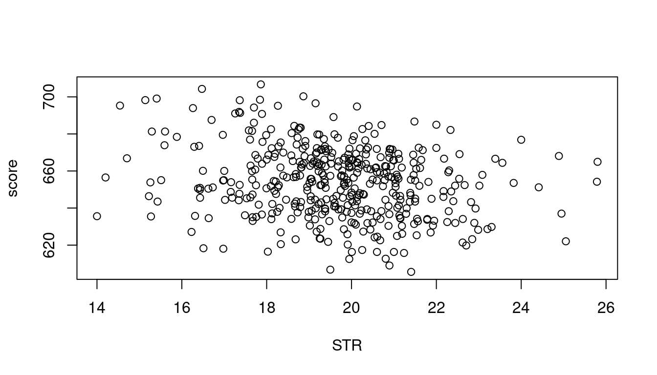
# Set up a plotting area with two plots side by side
par(mfrow = c(1,2))
# Scatterplots of score vs. income and score vs. english
plot(score ~ income, data = mydata)
plot(score ~ english, data = mydata)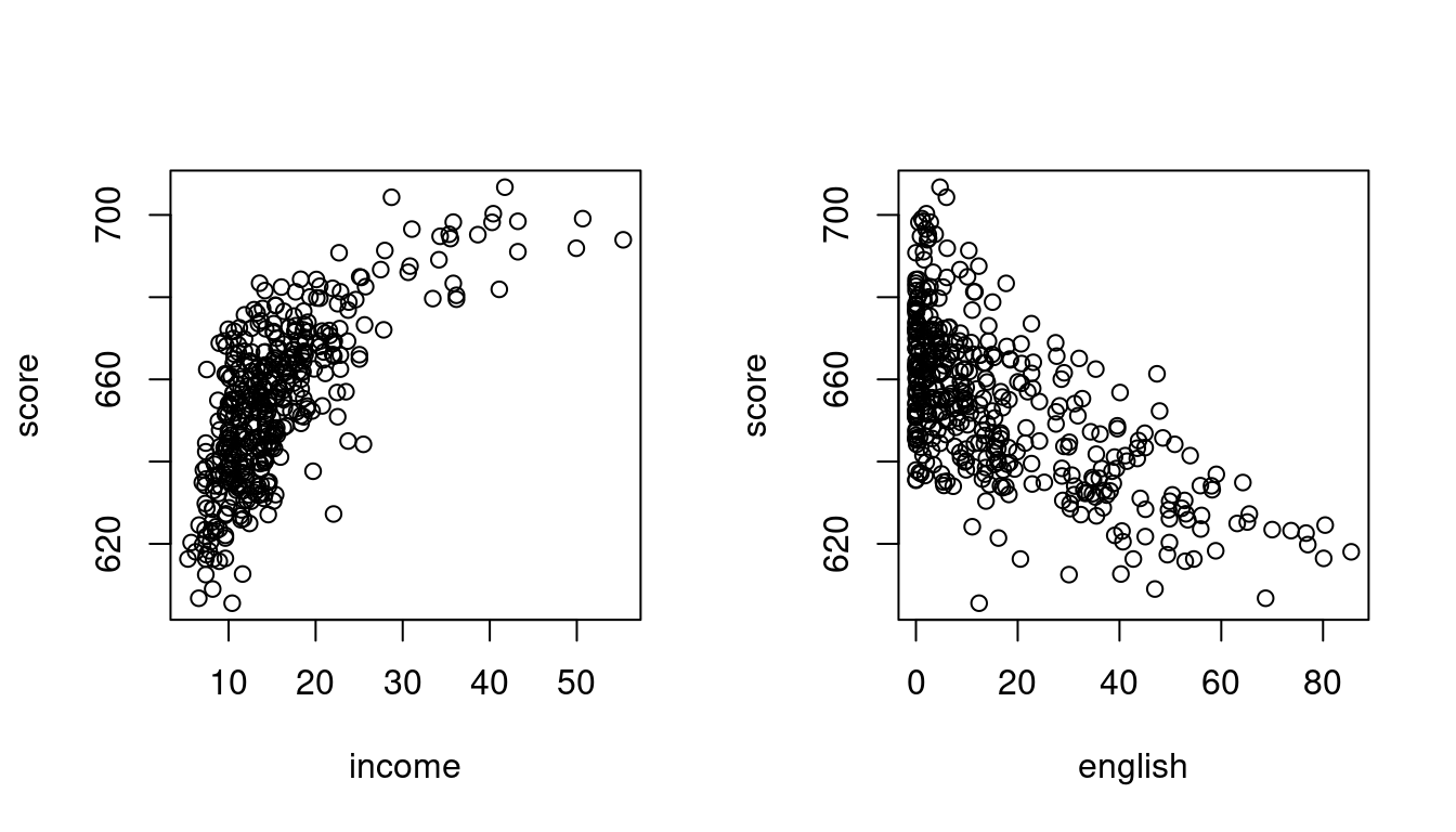
The option par(mfrow = c(1,2)) allows us to display multiple plots side by side. Try what happens if you replace c(1,2) with c(2,1).
1.4 Importing Data
The internet serves as a vast repository for data in various formats, with csv (comma-separated values), xlsx (Microsoft Excel spreadsheets), and txt (text files) being the most commonly used.
R supports various functions for different data formats:
-
read.csv()for reading comma-separated values -
read.csv2()for semicolon-separated values (adopting the German data convention of using the comma as the decimal mark) -
read.table()for whitespace-separated files -
read_excel()for Microsoft Excel files (requires thereadxlpackage) -
read_stata()for STATA files (requires thehavenpackage)
CPS Dataset
Let’s import the CPS dataset from Bruce Hansen’s textbook Econometrics.
The Current Population Survey (CPS) is a monthly survey conducted by the U.S. Census Bureau for the Bureau of Labor Statistics, primarily used to measure the labor force status of the U.S. population.
- Dataset: cps09mar.txt
- Description: cps09mar_description.pdf
url = "https://users.ssc.wisc.edu/~bhansen/econometrics/cps09mar.txt"
varnames = c("age", "female", "hisp", "education", "earnings", "hours",
             "week", "union", "uncov", "region", "race", "marital")
cps = read.table(url, col.names = varnames)
Let’s create additional variables:
# wage per hour
cps$wage = cps$earnings/(cps$week * cps$hours)
# years since graduation
cps$experience = (cps$age - cps$education - 6)
# married dummy
cps$married = cps$marital %in% c(1, 2) |> as.numeric()
# Black dummy
cps$Black = (cps$race %in% c(2, 6, 10, 11, 12, 15, 16, 19)) |> as.numeric()
# Asian dummy
cps$Asian = (cps$race %in% c(4, 8, 11, 13, 14, 16, 17, 18, 19)) |> as.numeric()
We will need the CPS dataset later, so it is a good idea to save the dataset to your computer:
write.csv(cps, "cps.csv", row.names = FALSE)This command saves the dataset to a file named cps.csv in your current working directory (you can check yours by running getwd()). It’s best practice to use an R Project for your course work so that all files (data, scripts, outputs) are stored in a consistent and organized folder structure.
To read the data back into R later, just type cps = read.csv("cps.csv").
1.5 Data Types
The most common types of economic data are:
Cross-sectional data: Data collected on many entities at a single point in time without regard to temporal changes.
Time series data: Data on a single entity collected over multiple time periods.
Panel data: Data collected on multiple entities over multiple time points, combining features of both cross-sectional and time series data.
Cross-Sectional Data
The cps dataset is an example of a cross-sectional dataset, as it contains observations from various individuals at a single point in time.
str(cps)Click here to view or hide the output
'data.frame':   50742 obs. of  20 variables:
 $ age       : int  52 38 38 41 42 66 51 49 33 52 ...
 $ female    : int  0 0 0 1 0 1 0 1 0 1 ...
 $ hisp      : int  0 0 0 0 0 0 0 0 0 0 ...
 $ education : int  12 18 14 13 13 13 16 16 16 14 ...
 $ earnings  : int  146000 50000 32000 47000 161525 33000 37000 37000 80000 32000 ...
 $ hours     : int  45 45 40 40 50 40 44 44 40 40 ...
 $ week      : int  52 52 51 52 52 52 52 52 52 52 ...
 $ union     : int  0 0 0 0 1 0 0 0 0 0 ...
 $ uncov     : int  0 0 0 0 0 0 0 0 0 0 ...
 $ region    : int  1 1 1 1 1 1 1 1 1 1 ...
 $ race      : int  1 1 1 1 1 1 1 1 1 1 ...
 $ marital   : int  1 1 1 1 1 5 1 1 1 1 ...
 $ experience: num  34 14 18 22 23 47 29 27 11 32 ...
 $ wage      : num  62.4 21.4 15.7 22.6 62.1 ...
 $ married   : num  1 1 1 1 1 0 1 1 1 1 ...
 $ college   : int  0 1 1 0 0 0 1 1 1 1 ...
 $ black     : int  0 0 0 0 0 0 0 0 0 0 ...
 $ asian     : int  0 0 0 0 0 0 0 0 0 0 ...
 $ Black     : num  0 0 0 0 0 0 0 0 0 0 ...
 $ Asian     : num  0 0 0 0 0 0 0 0 0 0 ...
Time Series
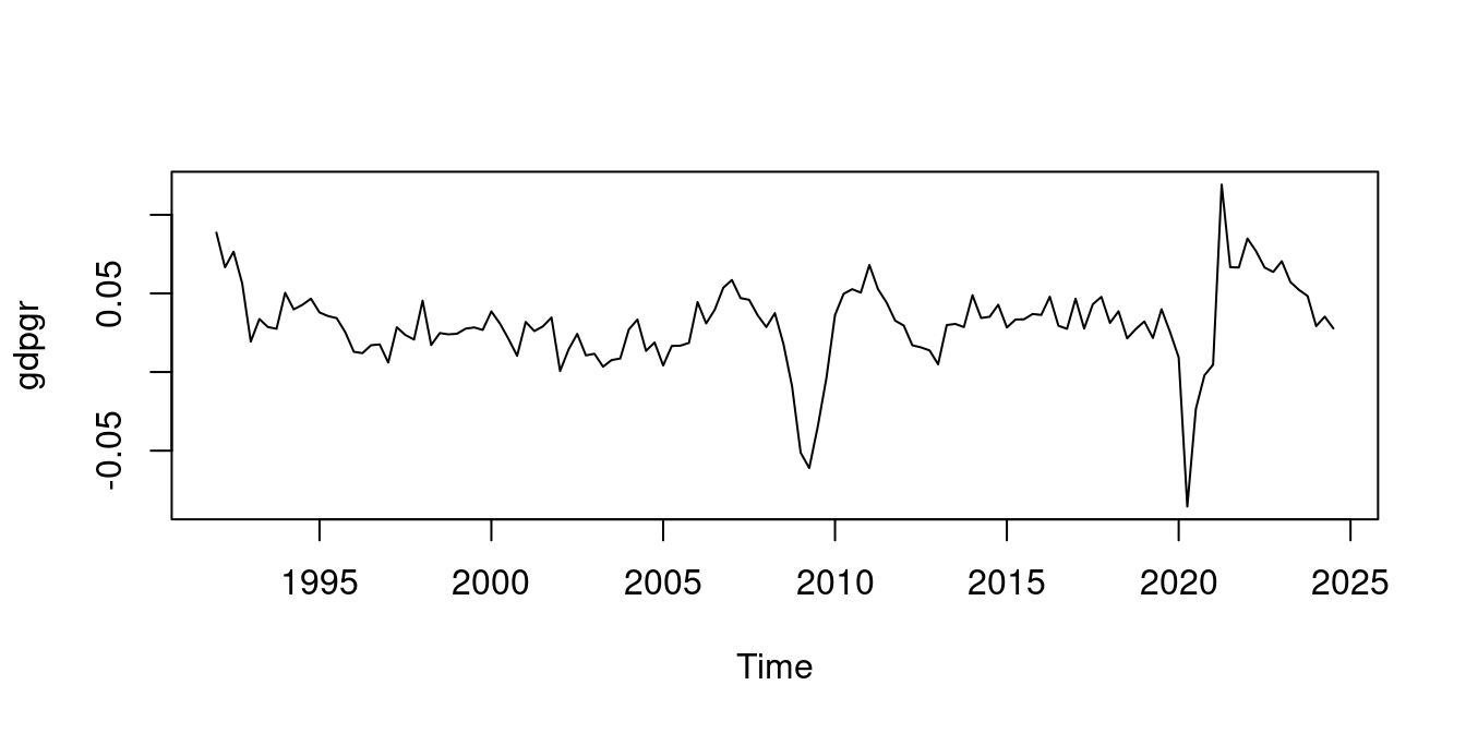
My repository TeachData contains several recent time series datasets. For instance, we can examine the annual growth rate of nominal quarterly GDP of Germany:
Panel Data
The dataset Fatalities is an example of a panel dataset. It contains variables related to traffic fatalities across different states (cross-sectional dimension) and years (time dimension) in the United States:
Click here to view or hide the output
'data.frame':   336 obs. of  34 variables:
 $ state       : Factor w/ 48 levels "al","az","ar",..: 1 1 1 1 1 1 1 2 2 2 ...
 $ year        : Factor w/ 7 levels "1982","1983",..: 1 2 3 4 5 6 7 1 2 3 ...
 $ spirits     : num  1.37 1.36 1.32 1.28 1.23 ...
 $ unemp       : num  14.4 13.7 11.1 8.9 9.8 ...
 $ income      : num  10544 10733 11109 11333 11662 ...
 $ emppop      : num  50.7 52.1 54.2 55.3 56.5 ...
 $ beertax     : num  1.54 1.79 1.71 1.65 1.61 ...
 $ baptist     : num  30.4 30.3 30.3 30.3 30.3 ...
 $ mormon      : num  0.328 0.343 0.359 0.376 0.393 ...
 $ drinkage    : num  19 19 19 19.7 21 ...
 $ dry         : num  25 23 24 23.6 23.5 ...
 $ youngdrivers: num  0.212 0.211 0.211 0.211 0.213 ...
 $ miles       : num  7234 7836 8263 8727 8953 ...
 $ breath      : Factor w/ 2 levels "no","yes": 1 1 1 1 1 1 1 1 1 1 ...
 $ jail        : Factor w/ 2 levels "no","yes": 1 1 1 1 1 1 1 2 2 2 ...
 $ service     : Factor w/ 2 levels "no","yes": 1 1 1 1 1 1 1 2 2 2 ...
 $ fatal       : int  839 930 932 882 1081 1110 1023 724 675 869 ...
 $ nfatal      : int  146 154 165 146 172 181 139 131 112 149 ...
 $ sfatal      : int  99 98 94 98 119 114 89 76 60 81 ...
 $ fatal1517   : int  53 71 49 66 82 94 66 40 40 51 ...
 $ nfatal1517  : int  9 8 7 9 10 11 8 7 7 8 ...
 $ fatal1820   : int  99 108 103 100 120 127 105 81 83 118 ...
 $ nfatal1820  : int  34 26 25 23 23 31 24 16 19 34 ...
 $ fatal2124   : int  120 124 118 114 119 138 123 96 80 123 ...
 $ nfatal2124  : int  32 35 34 45 29 30 25 36 17 33 ...
 $ afatal      : num  309 342 305 277 361 ...
 $ pop         : num  3942002 3960008 3988992 4021008 4049994 ...
 $ pop1517     : num  209000 202000 197000 195000 204000 ...
 $ pop1820     : num  221553 219125 216724 214349 212000 ...
 $ pop2124     : num  290000 290000 288000 284000 263000 ...
 $ milestot    : num  28516 31032 32961 35091 36259 ...
 $ unempus     : num  9.7 9.6 7.5 7.2 7 ...
 $ emppopus    : num  57.8 57.9 59.5 60.1 60.7 ...
 $ gsp         : num  -0.0221 0.0466 0.0628 0.0275 0.0321 ...
1.6 Statistical Framework
Data is usually the result of a random experiment. The gender of the next person you meet, the daily fluctuation of a stock price, the monthly music streams of your favorite artist, the annual number of pizzas consumed - all of this information involves a certain amount of randomness.
Random Variables
In statistical sciences, we interpret a univariate dataset Y_1, \ldots, Y_n as a sequence of random variables. Similarly, a multivariate dataset \boldsymbol X_1, \ldots, \boldsymbol X_n is viewed as a sequence of random vectors.
Cross-sectional data is typically characterized by an identical distribution across its individual observations, meaning each element in the sequence Y_1, \ldots, Y_n or \boldsymbol X_1, \ldots, \boldsymbol X_n has the same distribution function.
For example, if Y_1, \ldots, Y_n represent the wage levels of different individuals in Germany, each Y_i is drawn from the same distribution F, which in this context is the wage distribution across the country.
Similarly, if \boldsymbol X_1, \ldots, \boldsymbol X_n are bivariate random variables containing wages and years of education for individuals, each \boldsymbol X_i follows the same bivariate distribution G, which is the joint distribution of wages and education levels.
Probability Theory
A primary goal of econometric methods and statistical inference is to gain insights about features of these true but unknown population distributions F or G using the available data.
Thus, a solid knowledge of probability theory is essential for econometric modeling. For a comprehensive recap on probability theory for econometricians, consider the following refresher:
Probability Theory for Econometricians:
Section 2 of the Stock and Watson book also provides a review of the most important concepts.
Random Sampling
Econometric methods require specific assumptions about sampling processes. The ideal approach is simple random sampling, where each individual has an equal chance of being selected independently. This produces observations that are both identically distributed and independently drawn - what we call independent and identically distributed (i.i.d.) random variables or simply a random sample.
i.i.d. Sample
An independently and identically distributed (i.i.d.) sample, or random sample, consists of a sequence of k-variate random vectors \boldsymbol X_1, \ldots, \boldsymbol X_n that:
Have the same probability distribution F (identically distributed), where F(\boldsymbol a) = P(\boldsymbol X_i \leq \boldsymbol a) for any i and \boldsymbol a \in \mathbb R^k
Are mutually independent, meaning their joint cumulative distribution function F_{\boldsymbol X_1, \ldots, \boldsymbol X_n}(\boldsymbol a_1, \ldots, \boldsymbol a_n) = P(\boldsymbol X_1 \leq \boldsymbol a_1, \ldots, \boldsymbol X_n \leq \boldsymbol a_n) factorizes completely: F_{\boldsymbol X_1, \ldots, \boldsymbol X_n}(\boldsymbol a_1, \ldots, \boldsymbol a_n) = F(\boldsymbol a_1) \cdot F(\boldsymbol a_2) \cdot \ldots \cdot F(\boldsymbol a_n) for all \boldsymbol a_1, \ldots, \boldsymbol a_n \in \mathbb R^k.
F is called the population distribution or data-generating process (DGP).
An equivalent representation of the i.i.d. property can be obtained using the conditional distribution function F_{\boldsymbol X_i|\boldsymbol X_j=\boldsymbol a_j}(\boldsymbol a_i) = P(\boldsymbol X_i \leq \boldsymbol a_i| \boldsymbol X_j = \boldsymbol a_j, j\neq i). Then, \boldsymbol X_1, \ldots, \boldsymbol X_n are i.i.d. if the conditional distributions equal the marginal distributions: F_{\boldsymbol X_i|\boldsymbol X_j=\boldsymbol a_j}(\boldsymbol a_i) = F_{\boldsymbol X_i}(\boldsymbol a_i) = F(\boldsymbol a_i) \quad \text{for all} \ i \ \text{and} \ \boldsymbol a_1, \ldots, \boldsymbol a_n \in \mathbb R^k.
For more details on independence see Probability Tutorial Part 1
The Current Population Survey (CPS) involves random interviews with individuals from the U.S. labor force and may be regarded as an i.i.d. sample. Methods that commonly yield i.i.d. sampling for economic cross-sectional datasets include:
- Survey sampling with appropriate randomization
- Administrative records with random selection
- Direct observation of randomly chosen subjects
- Web scraping with randomized targets
- Field or laboratory experiments with random assignment
In a random sample there is no inherent ordering that would introduce systematic dependencies between observations. If individuals i and j are truly randomly selected, then the observations \boldsymbol X_i and \boldsymbol X_j are independent random vectors. The order in which the observations appear in the dataset is arbitrary and carries no information.
Clustered Sampling
While simple random sampling provides a clean theoretical foundation, real-world data often exhibits clustering - where observations are naturally grouped or nested within larger units. This clustering leads to dependencies that violate the i.i.d. assumption in two important contexts:
In cross-sectional studies, clustering occurs when we collect data on individual units that belong to distinct groups. Consider a study on student achievement where researchers randomly select schools, then collect data from all students within those schools:
- Although schools might be selected independently, observations at the student level are dependent
- Students within the same school share common environments (facilities, resources, administration)
- They experience similar teaching quality and educational policies and they influence each other through peer effects and social interactions
For instance, if School A has an exceptional mathematics department, all students from that school may perform better in math tests compared to students with similar abilities in other schools.
Statistically, if Y_{ik} represents the test score of student k in school i:
- observations Y_{ik} and Y_{jl} are independent for i \neq j (different students in different schools),
- observations Y_{ik} and Y_{il}are dependent (different students in the same school).
Panel Data Clustering
Panel data, by its very nature, introduces clustering across both cross-sectional units and time. Recall the Fatalities dataset which tracks traffic fatalities across different states and years.
For panel data with n states observed over T years, we can represent the structure as:
- The vectors (Y_{i1}, \ldots, Y_{iT}) are i.i.d. across units i=1,\ldots,n (different states’ time series are independently sampled)
- But within each state i, the observations Y_{i1}, \ldots, Y_{iT} are generally not independent from each other
This structure reflects two important aspects of panel data:
- Unit independence: The complete time series for each state can be treated as an independent draw from the population distribution of all possible state time series
- Temporal dependence: Within each state, observations across different years are dependent due to persistent state-specific factors like road infrastructure, driving culture, and enforcement practices
For instance, if California implements effective traffic safety measures, the effects will likely persist across multiple years, creating a temporal correlation in that state’s fatality rates. Similarly, economic downturns or changes in federal transportation policy may create dependencies across all states in particular years.
Time Dependence
Time series and panel data are intrinsically not independent due to the sequential nature of the observations. We usually expect observations close in time to be strongly dependent and observations at greater temporal distances to be less dependent.
Consider the quarterly GDP growth rates for Germany in the dataset gdpgr. Unlike cross-sectional data where the ordering of observations is arbitrary, the chronological ordering in time series carries crucial information about the dependency structure.
A simple way to formalize this temporal dependence is using an autoregression. If Y_t denotes the GDP growth at time t, a first-order autoregressive representation can be written as:
Y_t = \phi_0 + \phi_1 Y_{t-1} + \varepsilon_t
where \phi_0 is a constant, \phi_1 captures the persistence from one period to the next, and \varepsilon_t is a random disturbance.
If \phi_1 \neq 0, the current value Y_t directly depends on its previous value Y_{t-1}. For GDP growth, \phi_1 is typically positive, indicating that strong growth in one quarter predicts stronger growth in the next quarter.
This time dependence means that the conditional distribution function differs from the marginal distribution:
F_{Y_t|Y_{t-1},Y_{t-2},...}(y_t|y_{t-1},y_{t-2},...) \neq F_{Y_t}(y_t)
In contrast to the i.i.d. case, where F_{Y_i|Y_j}(y_i|y_j) = F_{Y_i}(y_i) for i \neq j, time series observations violate this independence property, making the i.i.d. assumption inappropriate for time series analysis.