Call:
lm(formula = wage ~ education, data = cps)

Coefficients:
(Intercept)    education
-16.448 2.898 4 Linear Model
4.1 Conditional Expectation
In econometrics, we often analyze how a variable of interest (like wages) varies systematically with other variables (like education or experience). The conditional expectation function (CEF) provides a powerful framework for describing these relationships.
The conditional expectation of Y given X is the expected value of Y for each possible value of X. For a continuous random variable Y we have E[Y|X = x] = \int_{-\infty}^\infty y \, f_{Y|X}(y|x) \, dy where f_{Y|X}(y|x) is the conditional density of Y given X = x.
The CEF maps values of X to corresponding conditional means of Y. As a function of the random variable X, the CEF itself is a random variable: E[Y|X] = m(X), \quad \text{where } m(x) = E[Y|X = x]
For a comprehensive treatment of conditional expectations see Probability Tutorial Part 2
Examples
Let’s examine this concept using wage and education as examples. When X is discrete (such as years of education), we can analyze how wage distributions change across education levels by comparing their conditional distributions:
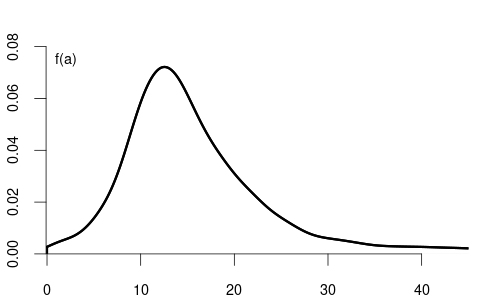
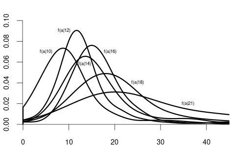
Notice how the conditional distributions shift rightward as education increases, indicating higher average wages with higher education.
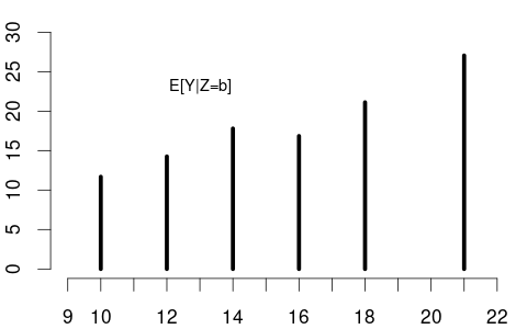
From these conditional densities, we can compute the expected wage for each education level. Plotting these conditional expectations gives the CEF: m(x) = E[\text{wage} \mid \text{edu} = x]
Since education is discrete, the CEF is defined only at specific values, as shown in the left plot below:
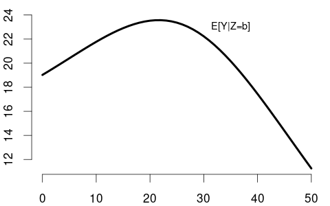
When X is continuous (like years of experience), the CEF becomes a smooth function (right plot). The shape of E[\text{wage}|\text{experience}] reflects real-world patterns: wages rise quickly early in careers, then plateau, and may eventually decline near retirement.
The CEF as a Random Variable
It’s important to distinguish between:
- E[Y|X = x]: a number (the conditional mean at a specific value)
- E[Y|X]: a function of X, which is itself a random variable
For instance, if X = \text{education} has the probability mass function: P(X = x) = \begin{cases} 0.06 & \text{if } x = 10 \\ 0.43 & \text{if } x = 12 \\ 0.16 & \text{if } x = 14 \\ 0.08 & \text{if } x = 16 \\ 0.24 & \text{if } x = 18 \\ 0.03 & \text{if } x = 21 \\ 0 & \text{otherwise} \end{cases}
Then E[Y|X] as a random variable has the probability mass function: P(E[Y|X] = y) = \begin{cases} 0.06 & \text{if } y = 11.68 \text{ (when } X = 10\text{)} \\ 0.43 & \text{if } y = 14.26 \text{ (when } X = 12\text{)} \\ 0.16 & \text{if } y = 17.80 \text{ (when } X = 14\text{)} \\ 0.08 & \text{if } y = 16.84 \text{ (when } X = 16\text{)} \\ 0.24 & \text{if } y = 21.12 \text{ (when } X = 18\text{)} \\ 0.03 & \text{if } y = 27.05 \text{ (when } X = 21\text{)} \\ 0 & \text{otherwise} \end{cases}
The CEF assigns to each value of X the expected value of Y given that information.
4.2 CEF Properties
The conditional expectation function has several important properties that make it a fundamental tool in econometric analysis.
Law of Iterated Expectations (LIE)
The law of iterated expectations connects conditional and unconditional expectations: E[Y] = E[E[Y|X]]
This means that to compute the overall average of Y, we can first compute the average of Y within each group defined by X, then average those conditional means using the distribution of X.
This is analogous to the law of total probability, where we compute marginal probabilities or densities as weighted averages of conditional ones:
When X is discrete: P(Y = y) = \sum_x P(Y = y \mid X = x) \cdot P(X = x)
When X is continuous: f_Y(y) = \int_{-\infty}^{\infty} f_{Y|X}(y \mid x) \cdot f_X(x) \, dx
Similarly, the LIE states:
When X is discrete: E[Y] = \sum_x E[Y \mid X = x] \cdot P(X = x)
When X is continuous: E[Y] = \int_{-\infty}^{\infty} E[Y \mid X = x] \cdot f_X(x) \, dx
Let’s apply this to our wage and education example. With X = \text{education} and Y = \text{wage}, we have:
\begin{aligned} E[Y|X=10] &= 11.68, \quad &P(X=10) = 0.06 \\ E[Y|X=12] &= 14.26, \quad &P(X=12) = 0.43 \\ E[Y|X=14] &= 17.80, \quad &P(X=14) = 0.16 \\ E[Y|X=16] &= 16.84, \quad &P(X=16) = 0.08 \\ E[Y|X=18] &= 21.12, \quad &P(X=18) = 0.24 \\ E[Y|X=21] &= 27.05, \quad &P(X=21) = 0.03 \end{aligned}
The law of iterated expectations gives us: \begin{aligned} E[Y] &= \sum_x E[Y|X = x] \cdot P(X = x) \\ &= 11.68 \cdot 0.06 + 14.26 \cdot 0.43 + 17.80 \cdot 0.16 \\ &\quad + 16.84 \cdot 0.08 + 21.12 \cdot 0.24 + 27.05 \cdot 0.03 \\ &= 0.7008 + 6.1318 + 2.848 + 1.3472 + 5.0688 + 0.8115 \\ &= 16.91 \end{aligned}
This unconditional expected wage of 16.91 aligns with what we would calculate from the unconditional density. The LIE provides us with a powerful way to bridge conditional expectations (within education groups) and the overall unconditional expectation (averaging across all education levels).
Conditioning Theorem (CT)
The conditioning theorem (also called the factorization rule) states: E[g(X)Y \mid X] = g(X) \cdot E[Y \mid X]
This means that when taking the conditional expectation of a product where one factor is a function of the conditioning variable, that factor can be treated as a constant and factored out. Once we condition on X, the value of g(X) is fixed.
If Y = \text{wage} and X = \text{education}, then for someone with 16 years of education: E[16 \cdot \text{wage} \mid \text{edu} = 16] = 16 \cdot E[\text{wage} \mid \text{edu} = 16]
More generally, if we want to find the expected product of education and wage, conditional on education: E[\text{edu} \cdot \text{wage} \mid \text{edu}] = \text{edu} \cdot E[\text{wage} \mid \text{edu}]
Best Predictor Property
The conditional expectation E[Y|X] is the best predictor of Y given X in terms of mean squared error: E[Y|X] = \arg\min_{g(\cdot)} E[(Y - g(X))^2]
This means that among all possible functions of X, the CEF minimizes the expected squared prediction error. In practical terms, if you want to predict wages based only on education, the optimal prediction is exactly the conditional mean wage for each education level.
For example, if someone has 18 years of education, our best prediction of their wage (minimizing expected squared error) is E[\text{wage}|\text{education}=18] = 21.12.
No other function of education, whether linear, quadratic, or more complex, can yield a better prediction in terms of expected squared error than the CEF itself.
Independence Implications
If Y and X are independent, then: E[Y|X] = E[Y]
When variables are independent, knowing X provides no information about Y, so the conditional expectation equals the unconditional expectation. The CEF becomes a constant function that doesn’t vary with X.
In our wage example, if education and wage were completely independent, the CEF would be a horizontal line at the overall average wage of 16.91. Each conditional density f_{Y|X}(y|x) would be identical to the unconditional density f(y), and the conditional means would all equal the unconditional mean.
The fact that our CEF for wage given education has a positive slope indicates that these variables are not independent—higher education is associated with higher expected wages.
4.3 Linear Model Specification
Prediction Error
Consider a sample \{(Y_i, \boldsymbol X_i)\}_{i=1}^n. We have established that the conditional expectation function (CEF) E[Y_i|\boldsymbol X_i] is the best predictor of Y_i given \boldsymbol X_i, minimizing the mean squared prediction error.
This leads to the following prediction error: u_i = Y_i - E[Y_i|\boldsymbol X_i]
By construction, this error has a conditional mean of zero: E[u_i | \boldsymbol X_i] = 0
This zero conditional mean property follows directly from the law of iterated expectations: \begin{align*} E[u_i | \boldsymbol X_i] &= E[Y_i - E[Y_i|\boldsymbol X_i] \mid \boldsymbol X_i] \\ &= E[Y_i \mid \boldsymbol X_i] - E[E[Y_i|\boldsymbol X_i] \mid \boldsymbol X_i] \\ &= E[Y_i \mid \boldsymbol X_i] - E[Y_i \mid \boldsymbol X_i] = 0 \end{align*}
We can thus always decompose the outcome as: Y_i = E[Y_i|\boldsymbol X_i] + u_i
where E[u_i|\boldsymbol X_i] = 0. This equation is not yet a regression model. It’s simply the decomposition of Y_i into its conditional expectation and an unpredictable component.
Linear Regression Model
To move to a regression framework, we impose a structural assumption about the form of the CEF. The key assumption of the linear regression model is that the conditional expectation is a linear function of the regressors: E[Y_i \mid \boldsymbol X_i] = \boldsymbol X_i'\boldsymbol \beta
Substituting this into our decomposition yields the linear regression equation: Y_i = \boldsymbol X_i'\boldsymbol \beta + u_i \tag{4.1}
with the crucial assumption: E[u_i \mid \boldsymbol X_i] = 0 \tag{4.2}
Exogeneity
This assumption (Equation 9.3) is called exogeneity or mean independence. It ensures that the linear function \boldsymbol X_i'\boldsymbol \beta correctly captures the conditional mean of Y_i.
Under the linear regression equation (Equation 4.1) we have the following equivalence: E[Y_i \mid \boldsymbol X_i] = \boldsymbol X_i'\boldsymbol \beta \quad \Leftrightarrow \quad E[u_i \mid \boldsymbol X_i] = 0
Therefore, the linear regression model in its most general form is characterized by the two conditions: linear regression equation (Equation 4.1) and exogenous regressors (Equation 9.3).
For example, in a wage regression, exogeneity means that the expected wage conditional on education and experience is exactly captured by the linear combination of these variables. No systematic pattern remains in the error term.
Model Misspecification
If the true conditional expectation function is nonlinear (e.g., if wages increase with education at a diminishing rate), then E[Y_i \mid \boldsymbol X_i] \neq \boldsymbol X_i'\boldsymbol \beta, and the model is misspecified. In such cases, the linear model provides the best linear approximation to the true CEF, but systematic patterns remain in the error term.
It’s important to note that u_i may still be statistically dependent on \boldsymbol X_i in ways other than its mean. For example, the variance of u_i may depend on \boldsymbol X_i in the case of heteroskedasticity. For instance, wage dispersion might increase with education level. The assumption E[u_i \mid \boldsymbol X_i] = 0 requires only that the conditional mean of the error is zero, not that the error is completely independent of the regressors.
4.4 Population Regression Coefficient
Under the linear model Y_i = \boldsymbol X_i'\boldsymbol \beta + u_i, \quad E[u_i \mid \boldsymbol X_i] = 0, we are interested in the population regression coefficient \boldsymbol \beta, which indicates how the conditional mean of Y_i varies linearly with the regressors in \boldsymbol X_i.
Moment Condition
A key implication of the exogeneity condition E[u_i \mid \boldsymbol X_i] = 0 is that the regressors are mean uncorrelated with the error term: E[\boldsymbol X_i u_i] = \boldsymbol 0
This can be derived from the exogeneity condition using the law of iterated expectations: E[\boldsymbol X_i u_i] = E[E[\boldsymbol X_i u_i \mid \boldsymbol X_i]] = E[\boldsymbol X_i \cdot E[u_i \mid \boldsymbol X_i]] = E[\boldsymbol X_i \cdot 0] = \boldsymbol 0
Substituting the linear model into the mean uncorrelatedness condition gives a moment condition that identifies \boldsymbol \beta: \boldsymbol 0 = E[\boldsymbol X_i u_i] = E[\boldsymbol X_i (Y_i - \boldsymbol X_i'\boldsymbol \beta)] = E[\boldsymbol X_i Y_i] - E[\boldsymbol X_i \boldsymbol X_i']\boldsymbol \beta
Rearranging to solve for \boldsymbol \beta: E[\boldsymbol X_i Y_i] = E[\boldsymbol X_i \boldsymbol X_i'] \boldsymbol \beta
Assuming that the matrix E[\boldsymbol X_i \boldsymbol X_i'] is invertible, we can express the population regression coefficient as: \boldsymbol \beta = \left(E[\boldsymbol X_i \boldsymbol X_i']\right)^{-1} E[\boldsymbol X_i Y_i]
This expression shows that \boldsymbol \beta is entirely determined by the joint distribution of (Y_i, \boldsymbol X_i') in the population.
The invertibility of E[\boldsymbol X_i \boldsymbol X_i'] is guaranteed if there is no perfect linear relationship among the regressors. In particular, no pair of regressors should be perfectly correlated, and no regressor should be a perfect linear combination of the other regressors.
OLS Estimation
To estimate \boldsymbol \beta from data, we replace population moments with sample moments. Given a sample \{(Y_i, \boldsymbol X_i)\}_{i=1}^n, the ordinary least squares (OLS) estimator is: \widehat{\boldsymbol \beta} = \left( \frac{1}{n} \sum_{i=1}^n \boldsymbol X_i \boldsymbol X_i' \right)^{-1} \left( \frac{1}{n} \sum_{i=1}^n \boldsymbol X_i Y_i \right)
This can be simplified to the familiar form: \widehat{\boldsymbol \beta} = (\boldsymbol X'\boldsymbol X)^{-1}\boldsymbol X'\boldsymbol Y
The OLS estimator solves the sample moment condition: \frac{1}{n} \sum_{i=1}^n \boldsymbol X_i (Y_i - \boldsymbol X_i'\widehat{\boldsymbol \beta}) = \boldsymbol 0
or equivalently: \frac{1}{n} \sum_{i=1}^n \boldsymbol X_i \widehat{u}_i = \boldsymbol 0
where \widehat{u}_i = Y_i - \boldsymbol X_i'\widehat{\boldsymbol \beta} are the sample residuals.
In this framework, OLS can be viewed as a method of moments estimator, solving the sample analogue of the population moment condition E[\boldsymbol X_i u_i] = \boldsymbol 0. The method of moments principle replaces theoretical moments with their empirical counterparts to obtain estimates of unknown parameters.
4.5 Marginal Effects
Consider the regression model of hourly wage on education (years of schooling), \text{wage}_i = \beta_1 + \beta_2 \text{edu}_i + u_i, \quad i=1, \ldots, n, where the exogeneity assumption holds: E[u_i | \text{edu}_i] = 0.
The population regression function, which gives the conditional expectation of wage given education, can be derived as: \begin{align*} m(\text{edu}_i) &= E[\text{wage}_i | \text{edu}_i] \\ &= \beta_1 + \beta_2 \cdot \text{edu}_i + E[u_i | \text{edu}_i] \\ &= \beta_1 + \beta_2 \cdot \text{edu}_i \end{align*}
Thus, the average wage level of all individuals with z years of schooling is: m(z) = \beta_1 + \beta_2 \cdot z.
Interpretation of Coefficients
In the linear regression model Y_i = \boldsymbol X_i'\boldsymbol \beta + u_i, the coefficient vector \boldsymbol \beta captures the way the conditional mean of Y_i changes with the regressors \boldsymbol X_i. Under the exogeneity assumption, E[Y_i \mid \boldsymbol X_i] = \boldsymbol X_i'\boldsymbol \beta = \beta_1 + \beta_2 X_{i2} + \ldots + \beta_k X_{ik}.
This linearity allows for a simple interpretation. The coefficient \beta_j represents the partial derivative of the conditional mean with respect to X_{ij}: \frac{\partial E[Y_i \mid \boldsymbol X_i]}{\partial X_{ij}} = \beta_j.
This means that \beta_j measures the marginal effect of a one-unit increase in X_{ij} on the expected value of Y_i, holding all other variables constant.
If X_{ij} is a dummy variable (i.e., binary), then \beta_j measures the discrete change in E[Y_i \mid \boldsymbol X_i] when X_{ij} changes from 0 to 1.
For our wage-education example, the marginal effect of education is: \frac{\partial E[\text{wage}_i | \text{edu}_i]}{\partial \text{edu}_i} = \beta_2.
This theoretical population parameter can be estimated using OLS:
Interpretation: People with one more year of education are paid on average $2.90 USD more per hour than people with one year less of education, assuming the exogeneity condition holds.
Correlation vs. Causation
The coefficient \beta_2 describes the correlative relationship between education and wages, not necessarily a causal one. To see this connection to correlation, consider the covariance of the two variables: \begin{align*} Cov(\text{wage}_i, \text{edu}_i) &= Cov(\beta_1 + \beta_2 \cdot \text{edu}_i + u_i, \text{edu}_i) \\ &= Cov(\beta_1 + \beta_2 \cdot \text{edu}_i, \text{edu}_i) + Cov(u_i, \text{edu}_i) \\ \end{align*}
The term Cov(u_i, \text{edu}_i) equals zero due to the exogeneity assumption. To see this, recall that E[u_i] = E[E[u_i|\text{edu}_i]] = 0 by the LIE and E[u_i \text{edu}_i] = 0 by mean uncorrelatedness, which implies Cov(u_i, \text{edu}_i) = E[u_i\text{edu}_i] - E[u_i] \cdot E[\text{edu}_i] = 0
The coefficient \beta_2 is thus proportional to the population correlation coefficient: \beta_2 = \frac{Cov(\text{wage}_i, \text{edu}_i)}{Var(\text{edu}_i)} = Corr(\text{wage}_i, \text{edu}_i) \cdot \frac{sd(\text{wage}_i)}{sd(\text{edu}_i)}.
The marginal effect is a correlative effect and does not necessarily reveal the source of the higher wage levels for people with more education.
Regression relationships do not necessarily imply causal relationships.
People with more education may earn more for various reasons:
- They might be naturally more talented or capable
- They might come from wealthier families with better connections
- They might have access to better resources and opportunities
- Education itself might actually increase productivity and earnings
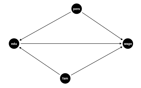
The coefficient \beta_2 measures how strongly education and earnings are correlated, but this association could be due to other factors that correlate with both wages and education, such as:
- Family background (parental education, family income, ethnicity)
- Personal background (gender, intelligence, motivation)
Omitted Variable Bias
To understand the causal effect of an additional year of education on wages, it is crucial to consider the influence of family and personal background. These factors, if not included in our analysis, are known as omitted variables. An omitted variable is one that:
- is correlated with the dependent variable (\text{wage}_i, in this scenario)
- is correlated with the regressor of interest (\text{edu}_i)
- is omitted in the regression
The presence of omitted variables means that we cannot be sure that the regression relationship between education and wages is purely causal. We say that we have omitted variable bias for the causal effect of the regressor of interest.
The coefficient \beta_2 in the simple regression model measures the correlative or marginal effect, not the causal effect. This must always be kept in mind when interpreting regression coefficients.
Control Variables
We can include control variables in the linear regression model to reduce omitted variable bias so that we can interpret \beta_2 as a ceteris paribus marginal effect (ceteris paribus means holding other variables constant).
For example, let’s include years of experience as well as racial background and gender dummy variables for Black and female: \text{wage}_i = \beta_1 + \beta_2 \text{edu}_i +\beta_3 \text{exper}_i + \beta_4 \text{Black}_i + \beta_5 \text{fem}_i + u_i.
In this case, \beta_2 = \frac{\partial E[\text{wage}_i | \text{edu}_i, \text{exper}_i, \text{Black}_i, \text{fem}_i]}{\partial \text{edu}_i} is the marginal effect of education on expected wages, holding experience, race, and gender fixed.
lm(wage ~ education + experience + Black + female, data = cps)
Call:
lm(formula = wage ~ education + experience + Black + female,
    data = cps)

Coefficients:
(Intercept)    education   experience        Black       female
   -21.7095       3.1350       0.2443      -2.8554      -7.4363
Interpretation of coefficients:
- Education: Given the same experience, racial background, and gender, people with one more year of education are paid on average $3.14 USD more than people with one year less of education.
- Experience: Each additional year of experience is associated with an average wage increase of $0.24 USD per hour, holding other factors constant.
- Black: Black workers earn on average $2.86 USD less per hour than non-Black workers with the same education, experience, and gender.
- Female: Women earn on average $7.43 USD less per hour than men with the same education, experience, and racial background.
Note: This regression does not control for other unobservable characteristics (such as ability) or variables not included in the regression (such as quality of education), so omitted variable bias may still be present.
Good vs. Bad Controls
It’s important to recognize that control variables are always selected with respect to a particular regressor of interest. A researcher typically focuses on estimating the effect of one specific variable (like education), and control variables must be designed specifically for this relationship.
In causal inference terminology, we can distinguish between different types of variables:
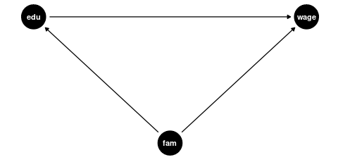
- Confounders: Variables that affect both the regressor of interest and the outcome. These are good controls because they help isolate the causal effect of interest.
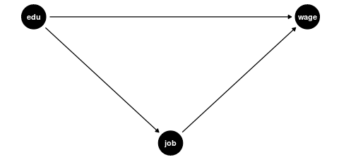
- Mediators: Variables through which the regressor of interest affects the outcome. Controlling for mediators can block part of the causal effect we’re trying to estimate.
- Colliders: Variables that are affected by both the regressor of interest and the outcome (or by factors that determine the outcome). Controlling for colliders can create spurious associations.
Confounders
Examples of good controls (confounders) for education are:
- Parental education level (affects both a person’s education and their wage potential)
- Region of residence (geographic factors can influence education access and job markets)
- Family socioeconomic background (affects educational opportunities and wage potential)
Mediators and Colliders
Examples of bad controls include:
-
Mediators: Variables that are part of the causal pathway from education to wages
- Current job position (education → job position → wage)
- Professional sector (education may determine which sector someone works in)
- Number of professional certifications (likely a result of education level)
-
Colliders: Variables affected by both education and wages (or their determinants)
- Happiness/life satisfaction (might be affected independently by both education and wages)
- Work-life balance (both education and wages might affect this independently)

Bad controls create two problems:
- Statistical issue: High correlation with the variable of interest (like education) causes high variance in the coefficient estimate (imperfect multicollinearity).
- Causal inference issue: They distort the relationship we’re trying to estimate by either blocking part of the causal effect (mediators) or creating artificial associations (colliders).
Good control variables are typically determined before the level of education is determined, while bad controls are often outcomes of the education process itself or are jointly determined with wages.
The appropriate choice of control variables requires not just statistical knowledge but also subject-matter expertise about the causal structure of the relationships being studied.
4.6 Application: Class Size Effect
Let’s apply these concepts to a real-world research question: How does class size affect student performance?
Recall the CASchools dataset used in the Stock and Watson textbook, which contains information on California school characteristics:
data(CASchools, package = "AER")
CASchools$STR = CASchools$students/CASchools$teachers
CASchools$score = (CASchools$read+CASchools$math)/2
We are interested in the effect of the student-teacher ratio STR (class size) on the average test score score. Following our previous discussion on causal inference, we need to consider potential confounding factors that might affect both class sizes and test scores.
Control Strategy
Let’s examine several control variables:
-
english: proportion of students whose primary language is not English. -
lunch: proportion of students eligible for free/reduced-price meals. -
expenditure: total expenditure per pupil.
First, we should check whether these variables are correlated with both our regressor of interest (STR) and the outcome (score):
                   STR      score     english       lunch expenditure
STR          1.0000000 -0.2263627  0.18764237  0.13520340 -0.61998216
score       -0.2263627  1.0000000 -0.64412381 -0.86877199  0.19127276
english      0.1876424 -0.6441238  1.00000000  0.65306072 -0.07139604
lunch        0.1352034 -0.8687720  0.65306072  1.00000000 -0.06103871
expenditure -0.6199822  0.1912728 -0.07139604 -0.06103871  1.00000000
The correlation matrix reveals that english, lunch, and expenditure are indeed correlated with both STR and score. This suggests they could be confounders that, if omitted, might bias our estimate of the class size effect.
Let’s implement a control strategy, adding potential confounders one by one to see how the estimated marginal effect of class size changes:
fit1 = lm(score ~ STR, data = CASchools)
fit2 = lm(score ~ STR + english, data = CASchools)
fit3 = lm(score ~ STR + english + lunch, data = CASchools)
fit4 = lm(score ~ STR + english + lunch + expenditure, data = CASchools)
library(modelsummary)
mymodels = list(fit1, fit2, fit3, fit4)
modelsummary(mymodels,
             statistic = NULL,
gof_map = c("nobs", "r.squared", "adj.r.squared", "rmse"))| (1) | (2) | (3) | (4) | |
|---|---|---|---|---|
| (Intercept) | 698.933 | 686.032 | 700.150 | 665.988 |
| STR | -2.280 | -1.101 | -0.998 | -0.235 |
| english | -0.650 | -0.122 | -0.128 | |
| lunch | -0.547 | -0.546 | ||
| expenditure | 0.004 | |||
| Num.Obs. | 420 | 420 | 420 | 420 |
| R2 | 0.051 | 0.426 | 0.775 | 0.783 |
| R2 Adj. | 0.049 | 0.424 | 0.773 | 0.781 |
| RMSE | 18.54 | 14.41 | 9.04 | 8.86 |
Interpretation of Marginal Effects
Let’s interpret the coefficients on STR from each model more precisely:
Model (1): Between two classes that differ by one student, the class with more students scores on average 2.280 points lower. This represents the unadjusted association without controlling for any confounding factors.
Model (2): Between two classes that differ by one student but have the same share of English learners, the larger class scores on average 1.101 points lower. Controlling for English learner status cuts the estimated effect by more than half.
Model (3): Between two classes that differ by one student but have the same share of English learners and students with reduced meals, the larger class scores on average 0.998 points lower. Adding this socioeconomic control further reduces the estimated effect slightly.
Model (4): Between two classes that differ by one student but have the same share of English learners, students with reduced meals, and per-pupil expenditure, the larger class scores on average 0.235 points lower. This represents a dramatic reduction from the previous model.
The sequential addition of controls demonstrates how sensitive the estimated marginal effect is to model specification. Each coefficient represents the partial derivative of the expected test score with respect to the student-teacher ratio, holding constant the variables included in that particular model.
Identifying Good and Bad Controls
Based on our causal framework from the previous section, we can evaluate our control variables:
Confounders (good controls):
englishandlunchare likely good controls because they represent pre-existing student characteristics that influence both class size assignments (schools might create smaller classes for disadvantaged students) and test performance.Mediator (bad control):
expenditureappears to be a bad control because it’s likely a mediator in the causal pathway from class size to test scores. Smaller classes mechanically increase per-pupil expenditure through higher teacher salary costs per student.
The causal relationship can be visualized as:
Class Size → Expenditure → Test Scores
When we control for expenditure, we block this causal pathway and “control away” part of the effect we actually want to measure. This explains the dramatic drop in the coefficient in Model (4) and suggests this model likely underestimates the true effect of class size.
This application demonstrates the crucial importance of thoughtful control variable selection in regression analysis. The estimated marginal effect of class size on test scores varies substantially depending on which variables we control for. Based on causal reasoning, we should prefer Model (3) with the appropriate confounders but without the mediator.
4.7 Nonlinear Modeling
Polynomials
A linear dependence on wages and experience is a strong assumption. We can reasonably expect a nonlinear marginal effect of another year of experience on wages. For example, the effect may be higher for workers with 5 years of experience than for those with 40 years of experience.
Polynomials can be used to specify a nonlinear regression function: \text{wage}_i = \beta_1 + \beta_2 \text{exper}_i + \beta_3 \text{exper}_i^2 + \beta_4 \text{exper}_i^3 + u_i.
## we focus on people with Asian background only for illustration
cps.as = cps |> subset(Asian == 1)
fit = lm(wage ~ experience + I(experience^2) + I(experience^3),
         data = cps.as)
beta = fit$coefficients
beta |> round(4)
(Intercept) experience I(experience^2) I(experience^3)
20.4547 1.2013 -0.0447 0.0004 ## Scatterplot
plot(wage ~ experience, data = cps.as, ylim = c(0,100))
## plot the cubic function for fitted wages
curve(
beta[1] + beta[2]*x + beta[3]*x^2 + beta[4]*x^3,
from = 0, to = 70, add=TRUE, col='red', lwd=2
)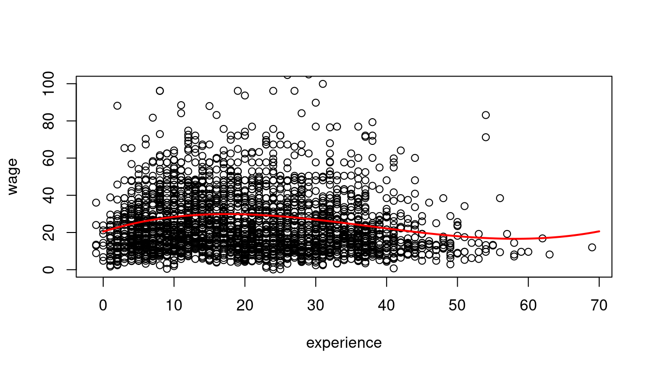
The marginal effect depends on the years of experience: \frac{\partial E[\text{wage}_i | \text{exper}_i] }{\partial \text{exper}_i} = \beta_2 + 2 \beta_3 \text{exper}_i + 3 \beta_4 \text{exper}_i^2. For instance, the additional wage for a worker with 11 years of experience compared to a worker with 10 years of experience is on average 1.2013 + 2\cdot (-0.0447) \cdot 10 + 3 \cdot 0.0004 \cdot 10^2 = 0.4273.
Interactions
A linear regression with interaction terms: \text{wage}_i = \beta_1 + \beta_2 \text{edu}_i + \beta_3 \text{fem}_i + \beta_4 \text{marr}_i + \beta_5 (\text{marr}_i \cdot \text{fem}_i) + u_i
lm(wage ~ education + female + married + married:female, data = cps)
Call:
lm(formula = wage ~ education + female + married + married:female,
    data = cps)

Coefficients:
   (Intercept)       education          female         married  female:married
       -17.886           2.867          -3.266           7.167          -5.767
The marginal effect of gender depends on the person’s marital status: \frac{\partial E[\text{wage}_i | \text{edu}_i, \text{fem}_i, \text{marr}_i] }{\partial \text{fem}_i} = \beta_3 + \beta_5 \text{marr}_i Interpretation: Given the same education, unmarried women are paid on average 3.27 USD less than unmarried men, and married women are paid on average 3.27+5.77=9.04 USD less than married men.
The marginal effect of the marital status depends on the person’s gender: \frac{\partial E[\text{wage}_i | \text{edu}_i, \text{fem}_i, \text{marr}_i]} {\partial \text{marr}_i} = \beta_4 + \beta_5 \text{fem}_i Interpretation: Given the same education, married men are paid on average 7.17 USD more than unmarried men, and married women are paid on average 7.17-5.77=1.40 USD more than unmarried women.
Logarithms
When analyzing wage data, we often use logarithmic transformations because they help model proportional relationships and reduce the skewness of the typically right-skewed distribution of wages. A common specification is the log-linear model, where we take the logarithm of wages while keeping education in its original scale:
In the logarithmic specification \log(\text{wage}_i) = \beta_1 + \beta_2 \text{edu}_i + u_i we have \frac{\partial E[\log(\text{wage}_i) | edu_i] }{\partial \text{edu}_i} = \beta_2.
This implies \underbrace{\partial E[\log(\text{wage}_i) | \text{edu}_i]}_{\substack{\text{absolute} \\ \text{change}}} = \beta_2 \cdot \underbrace{\partial \text{edu}_i}_{\substack{\text{absolute} \\ \text{change}}}. That is, \beta_2 gives the average absolute change in log-wages when education changes by 1.
Another interpretation can be given in terms of relative changes. Consider the following approximation: E[\text{wage}_i | \text{edu}_i] \approx \exp(E[\log(\text{wage}_i) | \text{edu}_i]). The left-hand expression is the conventional conditional mean, and the right-hand expression is the geometric mean. The geometric mean is slightly smaller because E[\log(Y)] < \log(E[Y]), but this difference is small unless the data is highly skewed.
The marginal effect of a change in edu on the geometric mean of wage is \frac{\partial exp(E[\log(\text{wage}_i) | \text{edu}_i])}{\partial \text{edu}_i} = \underbrace{exp(E[\log(\text{wage}_i) | \text{edu}_i])}_{\text{outer derivative}} \cdot \beta_2. Using the geometric mean approximation from above, we get \underbrace{\frac{\partial E[\text{wage}_i| \text{edu}_i] }{E[\text{wage}_i| \text{edu}_i]}}_{\substack{\text{percentage} \\ \text{change}}} \approx \frac{\partial exp(E[\log(\text{wage}_i) | \text{edu}_i])}{exp(E[\log(\text{wage}_i) | \text{edu}_i])} = \beta_2 \cdot \underbrace{\partial \text{edu}_i}_{\substack{\text{absolute} \\ \text{change}}}.
linear_model = lm(wage ~ education, data = cps.as)
log_model = lm(log(wage) ~ education, data = cps.as)
log_model
Call:
lm(formula = log(wage) ~ education, data = cps.as)

Coefficients:
(Intercept)    education
1.3783 0.1113 plot(wage ~ education, data = cps.as, ylim = c(0,80), xlim = c(4,22))
abline(linear_model, col="blue")
coef = coefficients(log_model)
curve(exp(coef[1]+coef[2]*x), add=TRUE, col="red")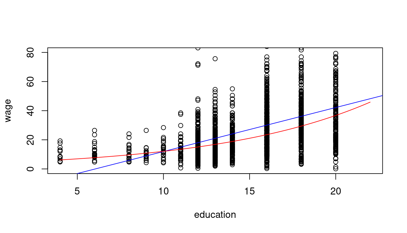
Interpretation: A person with one more year of education has a wage that is 11.13% higher on average.
In addition to the linear-linear and log-linear specifications, we also have the linear-log specification Y = \beta_1 + \beta_2 \log(X) + u and the log-log specification \log(Y) = \beta_1 + \beta_2 \log(X) + u.
Linear-log interpretation: When X is 1\% higher, we observe, on average, a 0.01 \beta_2 higher Y.
Log-log interpretation: When X is 1\% higher, we observe, on average, a \beta_2 \% higher Y.