(Intercept)   education      female
-14.081788 2.958174 -7.533067 5 Regression Inference
Recall the linear regression framework. We observe a sample \{(\boldsymbol{X}_i, Y_i)\}_{i=1}^n and assume Y_i = \boldsymbol{X}_i' \boldsymbol{\beta} + u_i, \quad E[u_i \mid \boldsymbol{X}_i] = 0,
where \boldsymbol{X}_i is a k-dimensional regressor vector (including an intercept), \boldsymbol{\beta} is the unknown parameter vector, and u_i is the error term. In matrix form we have \boldsymbol Y = \boldsymbol X \boldsymbol \beta + \boldsymbol u, where \boldsymbol{X} is the n \times k design matrix (its rows are: \boldsymbol{X}_i'), \boldsymbol{Y} is the n-vector of dependent variables, and \boldsymbol u is the n-vector of errors.
The OLS estimator \widehat{\boldsymbol{\beta}} is obtained by minimizing the sum of squared residuals: \begin{align*} \widehat{\boldsymbol{\beta}} &= \arg\min_{\boldsymbol{b}} \sum_{i=1}^n (Y_i - \boldsymbol{X}_i' \boldsymbol{b})^2 \\ &=\Big( \sum_{i=1}^n \boldsymbol X_i \boldsymbol X_i' \Big)^{-1} \sum_{i=1}^n \boldsymbol X_i Y_i \\ &= (\boldsymbol{X}'\boldsymbol{X})^{-1}\,(\boldsymbol{X}'\boldsymbol{Y}). \end{align*}
5.1 Strict Exogeneity
The weak exogeneity condition
E[u_i \mid \boldsymbol{X}_i] = 0
ensures that the regressors are uncorrelated with the error at the individual observation level. However, this condition is not sufficient to guarantee that the OLS estimator is unbiased. It still allows for u_i to be correlated with regressors from other observations (\boldsymbol{X}_j for j \ne i), which can lead to a biased estimation.
To ensure unbiasedness, we require the stronger condition of strict exogeneity: E[u_i \mid \boldsymbol{X}_j] = 0 \quad \text{for each } j = 1, \ldots, n, or, equivalently in matrix form: E[\boldsymbol{u} \mid \boldsymbol{X}] = \boldsymbol{0}.
Strict exogeneity requires the entire vector of errors \boldsymbol{u} to be mean independent of the full regressor matrix \boldsymbol{X}. That is, no systematic relationship exists between any regressors and any error term across observations.
Note
Under i.i.d. sampling, strict exogeneity typically holds automatically: independence across observations ensures u_i is uncorrelated with \boldsymbol{X}_j for j \ne i.
However, strict exogeneity may fail in dynamic time series settings, e.g.:
Y_t = \beta_1 + \beta_2 Y_{t-1} + u_t, \quad E[u_t|Y_{t-1}] = 0. \tag{5.1} Here, u_t is uncorrelated with Y_{t-1}, but it is correlated through Equation 5.1 with Y_t, which is the regressor for the dependent variable Y_{t+1}: Y_{t+1} = \beta_1 + \beta_2 Y_t + u_{t+1}, \quad E[u_{t+1}|Y_t] = 0. \tag{5.2} Therefore the error of Equation 5.1 is correlated with the regressor of Equation 5.2, violating strict exogeneity.
5.2 Unbiasedness
To derive the unbiasedness of the OLS estimator, recall the model: \boldsymbol{Y} = \boldsymbol{X}\boldsymbol{\beta} + \boldsymbol{u}.
Plugging this into the OLS formula: \begin{align*} \widehat{\boldsymbol{\beta}} &= (\boldsymbol{X}'\boldsymbol{X})^{-1} \boldsymbol{X}'\boldsymbol{Y} \\ &= (\boldsymbol{X}'\boldsymbol{X})^{-1} \boldsymbol{X}'(\boldsymbol{X} \boldsymbol{\beta} + \boldsymbol{u}) \\ &= \boldsymbol{\beta} + (\boldsymbol{X}'\boldsymbol{X})^{-1} \boldsymbol{X}'\boldsymbol{u}. \end{align*}
Taking the conditional expectation: E[\widehat{\boldsymbol{\beta}} \mid \boldsymbol{X}] = \boldsymbol{\beta} + (\boldsymbol{X}'\boldsymbol{X})^{-1} \boldsymbol{X}' E[\boldsymbol{u} \mid \boldsymbol{X}].
Under strict exogeneity, E[\boldsymbol{u} \mid \boldsymbol{X}] = \boldsymbol{0}, so: E[\widehat{\boldsymbol{\beta}} \mid \boldsymbol{X}] = \boldsymbol{\beta}.
Taking the expectation over the sampling distribution of \boldsymbol{X}: E[\widehat{\boldsymbol{\beta}}] = E[E[\widehat{\boldsymbol{\beta}} \mid \boldsymbol{X}]] = \boldsymbol{\beta}.
Thus, each element of the OLS estimator is unbiased: E[\widehat{\beta}_j] = \beta_j \quad \text{for } j = 1, \ldots, k.
Under strict exogeneity, the OLS estimator \widehat{\boldsymbol{\beta}} is unbiased: E[\widehat{\boldsymbol{\beta}}] = \boldsymbol{\beta}.
Even when strict exogeneity fails (as in time-dependent settings) asymptotic unbiasedness may still hold:
\lim_{n \to \infty} E[\widehat{\boldsymbol{\beta}}] = \boldsymbol \beta. For time series regressions, OLS remains asymptotically unbiased if far distant future regressors are independent of current errors, and the underlying relationship remains stable over time, i.e., there are no structural changes in the conditional mean function over time.
5.3 Sampling Variance of OLS
The OLS estimator \widehat{\boldsymbol \beta} provides a point estimate of the unknown population parameter \boldsymbol \beta. For example, in the regression \text{wage}_i = \beta_1 + \beta_2 \text{edu}_i + \beta_3 \text{fem}_i + u_i, we obtain specific coefficient estimates:
The estimate for education is \widehat \beta_2 = 2.958. However, this point estimate tells us nothing about how far it might be from the true value \beta_2. That is, it does not reflect estimation uncertainty, which arises because \widehat{\boldsymbol \beta} depends on a finite sample that could have turned out differently.
Larger samples tend to reduce estimation uncertainty, but in practice we only observe one finite sample. To quantify this uncertainty, we study the sampling variance of the OLS estimator: Var(\widehat{\boldsymbol \beta} \mid \boldsymbol X), the conditional variance of \widehat{\boldsymbol \beta} given the regressor matrix \boldsymbol X.
General formula for sampling variance of OLS:
Let \boldsymbol D = Var(\boldsymbol u \mid \boldsymbol X) be the conditional covariance matrix of the error terms. Then, Var(\widehat{\boldsymbol \beta} \mid \boldsymbol X) = (\boldsymbol X'\boldsymbol X)^{-1} \boldsymbol X' \boldsymbol D \boldsymbol X (\boldsymbol X'\boldsymbol X)^{-1}
This follows from \widehat{\boldsymbol{\beta}} = \boldsymbol{\beta} + (\boldsymbol{X}'\boldsymbol{X})^{-1} \boldsymbol{X}'\boldsymbol{u} together with the general rule that for any matrix \boldsymbol A, Var(\boldsymbol A \boldsymbol u) = \boldsymbol A \, Var(\boldsymbol u) \, \boldsymbol A'.
Depending on the structure of the data and the behavior of the error term, this expression takes different forms:
Homoskedasticity
Let \{(\boldsymbol X_i, Y_i)\}_{i=1}^n be an i.i.d. sample and let the error term be homoskedastic, meaning
Var(u_i \mid \boldsymbol X_i) = \sigma^2 \quad \text{for all } i.
Homoskedasticity means that the variance of the error does not depend on the value of the regressor. For instance, in a regression of wage on female, homoskedasticity means that men and women have the same error variance. Homoskedasticity holds if the error u_i is independent of the regressor \boldsymbol X_i.
The homoskedastic error covariance matrix has the following simple form: \boldsymbol{D} = \sigma^2 \boldsymbol{I}_n = \begin{pmatrix} \sigma^2 & 0 & \cdots & 0 \\ 0 & \sigma^2 & \cdots & 0 \\ \vdots & \vdots & \ddots & \vdots \\ 0 & 0 & \cdots & \sigma^2 \end{pmatrix}.
In this case, the sampling variance simplifies to: Var(\widehat{\boldsymbol \beta} \mid \boldsymbol X) = \sigma^2 (\boldsymbol X'\boldsymbol X)^{-1}.
This is the Gauss-Markov setting, in which OLS is the Best Linear Unbiased Estimator (BLUE).
Heteroskedasticity
If the sample is i.i.d., but Var(u_i \mid \boldsymbol X_i) depends on \boldsymbol X_i, the errors are heteroskedastic: Var(u_i \mid \boldsymbol X_i) = \sigma^2(\boldsymbol X_i) = \sigma_i^2.
For instance, in a regression of wage on gender, the wage variability might differ between men and women.
In this case, \boldsymbol D remains diagonal but no longer proportional to the identity matrix: \boldsymbol D = \begin{pmatrix} \sigma_1^2 & 0 & \cdots & 0 \\ 0 & \sigma_2^2 & \cdots & 0 \\ \vdots & \vdots & \ddots & \vdots \\ 0 & 0 & \cdots & \sigma_n^2 \end{pmatrix}.
The sampling variance becomes: Var(\widehat{\boldsymbol \beta} \mid \boldsymbol X) = (\boldsymbol X'\boldsymbol X)^{-1} \left[\sum_{i=1}^n \sigma_i^2 \boldsymbol X_i \boldsymbol X_i'\right] (\boldsymbol X'\boldsymbol X)^{-1}.
Clustered Sampling
For clustered observations we can use the notation (\boldsymbol X_{ig}, Y_{ig}) for i=1, \ldots, n_g observations in cluster g=1, \ldots, G: Y_{ig} = \boldsymbol X_{ig}' \boldsymbol \beta + u_{ig}, \quad i=1, \ldots, n_g, \quad g=1, \ldots, G.
We assume:
Weak exogeneity within clusters: E[u_{ig}\mid \boldsymbol X_{g}] = 0 for all g=1, \ldots, G.
Independence across clusters: (\boldsymbol Y_{1g}, \ldots, Y_{n_g g}, \boldsymbol X_{1g}', \ldots, \boldsymbol X_{n_g g}') are i.i.d. for g=1, \ldots, G.
This together ensures strict exogenity and unbiasedness of OLS, but allow for arbitrary correlation of errors within each cluster. The covariance matrix \boldsymbol D has a block-diagonal form: \boldsymbol D = \begin{pmatrix} \boldsymbol D_1 & 0 & \cdots & 0 \\ 0 & \boldsymbol D_2 & \cdots & 0 \\ \vdots & \vdots & \ddots & \vdots \\ 0 & 0 & \cdots & \boldsymbol D_G \end{pmatrix}, where each block \boldsymbol D_g is an n_g \times n_g matrix capturing the error covariances within cluster g: \boldsymbol D_g = \begin{pmatrix} E[u_{1g}^2|\boldsymbol X] & E[u_{1g}u_{2g}|\boldsymbol X] & \cdots & E[u_{1g}u_{n_gg}|\boldsymbol X] \\ E[u_{2g}u_{1g}|\boldsymbol X] & E[u_{2g}^2|\boldsymbol X] & \cdots & E[u_{2g}u_{n_gg}|\boldsymbol X] \\ \vdots & \vdots & \ddots & \vdots \\ E[u_{n_gg}u_{1g}|\boldsymbol X] & E[u_{n_gg}u_{2g}|\boldsymbol X] & \cdots & E[u_{n_gg}^2|\boldsymbol X] \end{pmatrix}. The middle part of the sandwich form of the covariance matrix Var(\widehat{\boldsymbol \beta} \mid \boldsymbol X) becomes: \boldsymbol X' \boldsymbol D \boldsymbol X = \sum_{g=1}^G E\bigg[ \Big( \sum_{i=1}^{n_g} \boldsymbol X_{ig} u_{ig} \Big) \Big( \sum_{i=1}^{n_g} \boldsymbol X_{ig} u_{ig} \Big)' \Big| \boldsymbol X \bigg].
Time Series Data
In time series regressions, errors u_t are often serially correlated. A typical example is an AR(1) process: u_t = \phi u_{t-1} + \varepsilon_t, where |\phi| < 1 and \varepsilon_t is i.i.d. with mean 0 and variance \sigma_\varepsilon^2.
Then the autocovariance structure is: Cov(u_t, u_{t-h}) = \sigma^2 \phi^h, \quad \text{for } h \geq 0, where \sigma^2 = \frac{\sigma_\varepsilon^2}{1 - \phi^2}.
The resulting covariance matrix \boldsymbol D has a Toeplitz structure: \boldsymbol D = \sigma^2 \begin{pmatrix} 1 & \phi & \phi^2 & \cdots & \phi^{n-1} \\ \phi & 1 & \phi & \cdots & \phi^{n-2} \\ \phi^2 & \phi & 1 & \cdots & \phi^{n-3} \\ \vdots & \vdots & \vdots & \ddots & \vdots \\ \phi^{n-1} & \phi^{n-2} & \phi^{n-3} & \cdots & 1 \end{pmatrix}.
5.4 Gaussian Regression
The Gaussian regression model builds on the linear regression framework by adding a distributional assumption. It assumes an i.i.d. sample and that the error terms are conditionally normally distributed: u_i \mid \boldsymbol{X}_i \sim \mathcal{N}(0, \sigma^2) \tag{5.3}
That is, conditional on the regressors, the error has mean zero (exogeneity), constant variance (homoskedasticity), and a normal distribution. This assumption implies that the OLS estimator itself is normally distributed, since it is a linear combination of normally distributed errors: \widehat{\boldsymbol{\beta}} \mid \boldsymbol{X} \sim \mathcal{N}(\boldsymbol{\beta}, \sigma^2(\boldsymbol{X}'\boldsymbol{X})^{-1}).
In particular, each standardized coefficient follows a standard normal distribution: \frac{\widehat \beta_j - \beta_j}{sd(\widehat \beta_j \mid \boldsymbol X)} \sim \mathcal{N}(0,1), with conditional standard deviation sd(\widehat \beta_j \mid \boldsymbol X) = \sigma \sqrt{(\boldsymbol{X}'\boldsymbol{X})^{-1}_{jj}}.
Classical Standard Errors
The conditional standard deviation of \widehat \beta_j is unknown because the population error variance \sigma^2 is unknown.
A standard error of \widehat \beta_j is an estimator of the conditional standard deviation. To construct a valid standard error under this setup, we can use the adjusted residual variance to estimate \sigma^2: s_{\widehat{u}}^2 = \frac{1}{n-k} \sum_{i=1}^n \widehat{u}_i^2. The classical standard error (valid under homoskedasticity) is defined as: se_{hom}(\widehat{\beta}_j) = s_{\widehat{u}} \sqrt{(\boldsymbol{X}'\boldsymbol{X})^{-1}_{jj}}.
Under the Gaussian assumption Equation 5.3, \widehat{\boldsymbol{\beta}} and s_{\widehat{u}}^2 are independent and s_{\widehat{u}}^2 has the following property: \frac{(n-k) s_{\widehat{u}}^2}{\sigma^2} \sim \chi^2_{n-k}. This allows us to derive the exact distribution of the standardized OLS coefficient when we replace the population standard deviation with its sample estimate (the standard error): \frac{\widehat \beta_j - \beta_j}{se_{hom}(\widehat \beta_j \mid \boldsymbol X)} = \frac{\widehat \beta_j - \beta_j}{sd(\widehat \beta_j \mid \boldsymbol X)} \cdot \frac{\sigma}{s_{\widehat{u}}} \sim \frac{\mathcal{N}(0,1)}{\sqrt{\chi^2_{n-k}/(n-k)}} = t_{n-k}
This means that the OLS coefficient standardized with the homoskedastic standard error instead of the standard deviation follows a t-distribution with n-k degrees of freedom.
For a refresher on the normal and t-distribution, see
Probability Tutorial Part 4
To estimate the full sampling covariance matrix Var(\widehat{\boldsymbol \beta} \mid \boldsymbol X), the classical covariance matrix estimator is: \widehat{\boldsymbol V}_{hom} = s_{\widehat u}^2 (\boldsymbol X'\boldsymbol X)^{-1}.
## classical homoskedastic covariance matrix estimator:
vcov(fit)
(Intercept) education female
(Intercept) 0.18825476 -0.0127486354 -0.0089269796
education -0.01274864 0.0009225111 -0.0002278021
female -0.00892698 -0.0002278021 0.0284200217Classical standard errors se_{hom}(\widehat{\beta}_j) are the square roots of the diagonal entries:
(Intercept)   education      female
 0.43388334  0.03037287  0.16858239
They are also displayed in parentheses in a typical regression summary table:
library(modelsummary)
modelsummary(fit, gof_map = "none")| (1) | |
|---|---|
| (Intercept) | -14.082 |
| (0.434) | |
| education | 2.958 |
| (0.030) | |
| female | -7.533 |
| (0.169) |
The argument gof_map = "none" omits all goodness of fit statistics like R-squared and RMSE.
Confidence Intervals
A confidence interval is a range of values that is likely to contain the true population parameter with a specified confidence level or coverage probability, often expressed as a percentage (e.g., 95%).
A (1 - \alpha) confidence interval for \beta_j is an interval I_{1-\alpha} such that P(\beta_j \in I_{1-\alpha}) = 1 - \alpha. Under the Gaussian assumption Equation 5.3, this property is satisfied for the classical homoskedastic confidence interval: I_{1-\alpha} = \bigg[ \widehat{\beta}_j - t_{n-k, 1-\alpha/2} \cdot se_{hom}(\widehat{\beta}_j); \widehat{\beta}_j + t_{n-k, 1-\alpha/2} \cdot se_{hom}(\widehat{\beta}_j) \bigg], where t_{n-k, 1-\alpha/2} is the 1-\alpha/2-quantile from the t-distribution with n-k degrees of freedom. Common coverage probabilities are 0.90, 0.95, 0.99, and 0.999.
| df | 0.95 | 0.975 | 0.995 | 0.9995 |
|---|---|---|---|---|
| 1 | 6.31 | 12.71 | 63.66 | 636.6 |
| 2 | 2.92 | 4.30 | 9.92 | 31.6 |
| 3 | 2.35 | 3.18 | 5.84 | 12.9 |
| 5 | 2.02 | 2.57 | 4.03 | 6.87 |
| 10 | 1.81 | 2.23 | 3.17 | 4.95 |
| 20 | 1.72 | 2.09 | 2.85 | 3.85 |
| 50 | 1.68 | 2.01 | 2.68 | 3.50 |
| 100 | 1.66 | 1.98 | 2.63 | 3.39 |
| \to \infty | 1.64 | 1.96 | 2.58 | 3.29 |
The last row (indicated by \to \infty) shows the quantiles of the standard normal distribution \mathcal N(0,1).
You can display 95% confidence intervals in the modelsummary output using the conf.int argument:
modelsummary(fit, gof_map = "none", statistic = "conf.int")| (1) | |
|---|---|
| (Intercept) | -14.082 |
| [-14.932, -13.231] | |
| education | 2.958 |
| [2.899, 3.018] | |
| female | -7.533 |
| [-7.863, -7.203] |
Note: the confidence interval is random, while the parameter \beta_j is fixed but unknown.

A correct interpretation of a 95% confidence interval is:
- If we were to repeatedly draw samples and construct a 95% confidence interval from each sample, about 95% of these intervals would contain the true parameter.
Common misinterpretations to avoid:
- ❌ “There is a 95% probability that the true value lies in this interval.”
- ❌ “We are 95% confident this interval contains the true parameter.”
These mistakes incorrectly treat the parameter as random and the interval as fixed. In reality, it’s the other way around.
A 95% confidence interval should be understood as a coverage probability: Before observing the data, there is a 95% probability that the random interval will cover the true parameter.
A helpful visualization:Limitations of the Gaussian Approach
The Gaussian regression framework assumes:
- Weak exogeneity: E[u_i \mid \boldsymbol X_i] = 0
- I.i.d. sample: \{(Y_i, \boldsymbol X_i)\}_{i=1}^n
- Homoskedastic, normally distributed errors: u_i|\boldsymbol X_i \sim \mathcal{N}(0, \sigma^2)
- \boldsymbol X'\boldsymbol X is invertible (i.e. \boldsymbol X has full rank)
While mathematically convenient, these assumptions are often violated in practice. In particular, the normality assumption implies homoskedasticity and that the conditional distribution of Y_i given \boldsymbol X_i is normal, which is an unrealistic scenario in many economic applications.
Historically, homoskedasticity has been treated as the “default” assumption and heteroskedasticity as a special case. But in empirical work, heteroskedasticity is the norm.
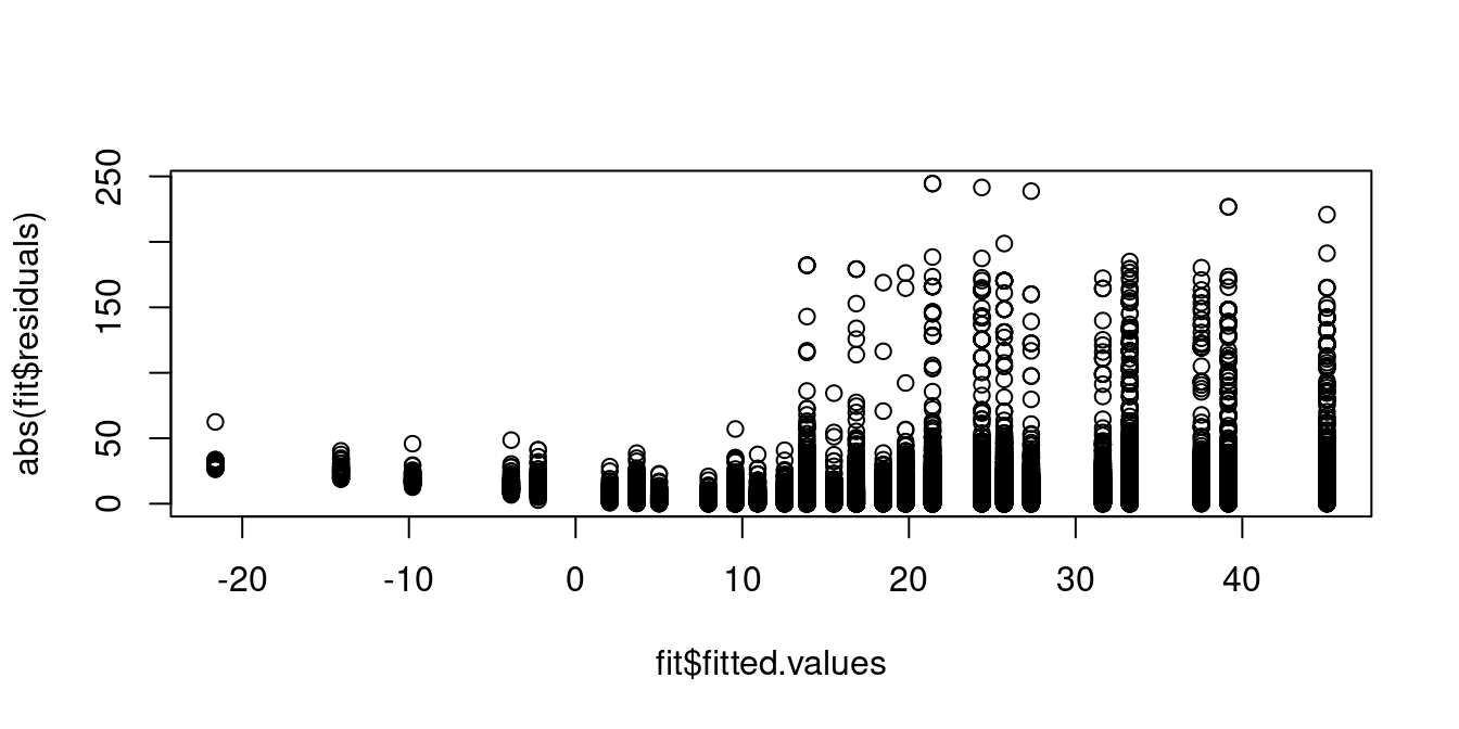
A plot of the absolute value of the residuals against the fitted values shows that individuals with predicted wages around 10 USD exhibit residuals with lower variance compared to those with higher predicted wage levels. Hence, the homoskedasticity assumption is implausible:
The Q-Q-plot is a graphical tool to help us assess if the errors are conditionally normally distributed.
Let \widehat u_{(i)} be the sorted residuals (i.e. \widehat u_{(1)} \leq \ldots \leq \widehat u_{(n)}). The Q-Q-plot plots the sorted residuals \widehat u_{(i)} against the ((i-0.5)/n)-quantiles of the standard normal distribution.
If the residuals are lined well on the straight dashed line, there is indication that the distribution of the residuals is close to a normal distribution.
set.seed(123)
par(mfrow = c(1,2))
## auxiliary regression with simulated normal errors:
fit.aux = lm(rnorm(500) ~ 1)
## Q-Q-plot of the residuals of the auxiliary regression:
qqnorm(residuals(fit.aux))
qqline(residuals(fit.aux))
## Q-Q-plot of the residuals of the wage regression:
qqnorm(residuals(fit))
qqline(residuals(fit))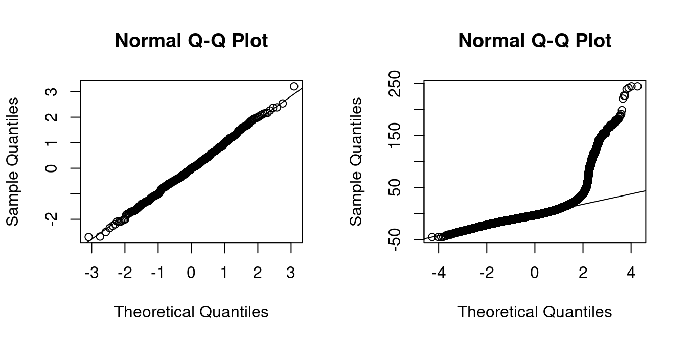
In the left plot you see the Q-Q-plot for an example with simulated normally distributed errors, where the Gaussian regression assumption is satisfied.
The right plot indicates that, in our regression of wage on education and female, the normality assumption is implausible.
5.5 Heteroskedastic Linear Model
The classical approach to regression relies on strong distributional assumptions: normality and homoskedasticity of the errors. While this enables exact inference in small samples, it is rarely justified in empirical applications.
The modern econometric approach avoids such assumptions and instead relies on asymptotic approximations under weaker conditions (i.e., finite kurtosis instead of normality and homoskedasticity).
Heteroskedastic Linear Model
We assume that the sample \{(Y_i, \boldsymbol X_i')\}_{i=1}^n satisfies the linear regression equation Y_i = \boldsymbol X_i'\boldsymbol \beta + u_i, \quad i=1, \ldots, n, under the following conditions:
-
(A1) E[u_i | \boldsymbol X_i] = 0 (weak exogeneity)
-
(A2) \{(Y_i, \boldsymbol X_i')\}_{i=1}^n is an i.i.d. sample (random sampling)
-
(A3) kur(Y_i) < \infty and kur(X_{ij}) < \infty for all j = 1, \ldots, k
(bounded kurtosis: large outliers are unlikely)
- (A4) \sum_{i=1}^n \boldsymbol X_i \boldsymbol X_i' is invertible (OLS is well defined)
Under heteroskedasticity, the error variance may depend on the regressor: \sigma_i^2 = \mathrm{Var}(u_i \mid \boldsymbol X_i), and the conditional standard deviation of \widehat \beta_j is sd(\widehat{\beta}_j \mid \boldsymbol X) = \sqrt{\bigg[(\boldsymbol{X}'\boldsymbol{X})^{-1} \Big(\sum_{i=1}^{n} \sigma_i^2 \boldsymbol{X}_i \boldsymbol{X}_i' \Big)(\boldsymbol{X}'\boldsymbol{X})^{-1}\bigg]_{jj}}. Unlike in the Gaussian case, the standardized OLS coefficient does not follow a standard normal distribution in finite samples: \frac{\widehat \beta_j - \beta_j}{sd(\widehat \beta_j \mid \boldsymbol X)} \nsim \mathcal{N}(0,1).
However, for large samples, the central limit theorem guarantees that the OLS estimator is asymptotically normal: \frac{\widehat \beta_j - \beta_j}{sd(\widehat \beta_j \mid \boldsymbol X)} \overset{d}{\rightarrow} \mathcal N(0,1) \quad \text{as } n \to \infty.
This result holds because the OLS estimator can be expressed as: \begin{align*} \sqrt n (\widehat{\boldsymbol \beta} - \boldsymbol \beta) &= \sqrt n\bigg( \sum_{i=1}^n \boldsymbol X_i \boldsymbol X_i' \bigg)^{-1} \sum_{i=1}^n \boldsymbol X_i u_i \\ &= \bigg( \frac{1}{n} \sum_{i=1}^n \boldsymbol X_i \boldsymbol X_i' \bigg)^{-1} \frac{1}{\sqrt{n}} \sum_{i=1}^n \boldsymbol X_i u_i, \end{align*} where:
- By the law of large numbers: \frac{1}{n} \sum_{i=1}^n \boldsymbol X_i \boldsymbol X_i' \overset{p}{\rightarrow} E[\boldsymbol X_i \boldsymbol X_i'] = \boldsymbol Q,
- And by the central limit theorem: \frac{1}{\sqrt{n}} \sum_{i=1}^n \boldsymbol X_i u_i \overset{d}{\rightarrow} \mathcal N(\boldsymbol 0, \boldsymbol \Omega), \quad \text{where } \boldsymbol \Omega = E[u_i^2 \boldsymbol X_i \boldsymbol X_i'].
For more details on stochastic convergence and the central limit theorem, see Probability Tutorial Part 4
Asymptotic Distribution of OLS Estimator
Under the heteroskedastic linear model: \sqrt{n}(\widehat{\boldsymbol \beta} - \boldsymbol \beta) \overset{d}{\to} \mathcal{N}(\boldsymbol{0},\; \boldsymbol Q^{-1} \boldsymbol \Omega \boldsymbol Q^{-1}), where \boldsymbol Q = E[\boldsymbol X_i \boldsymbol X_i'] and \boldsymbol \Omega = E[u_i^2 \boldsymbol X_i \boldsymbol X_i'].
This asymptotic distribution forms the basis for heteroskedasticity-robust inference.
5.6 Heteroskedasticity-Robust Standard Errors
The asymptotic distribution of the OLS estimator under heteroskedasticity depends on two population matrices:
-
\boldsymbol{Q} = E[\boldsymbol{X}_i \boldsymbol{X}_i'], and
- \boldsymbol{\Omega} = E[u_i^2 \boldsymbol{X}_i \boldsymbol{X}_i']
While \boldsymbol{Q} can be consistently estimated by its sample counterpart, \widehat{\boldsymbol{Q}} = \frac{1}{n} \sum_{i=1}^n \boldsymbol{X}_i \boldsymbol{X}_i', estimating \boldsymbol{\Omega} is more challenging because the error terms u_i are unobserved.
To overcome this, we replace the unobserved u_i with the OLS residuals: \widehat{u}_i = Y_i - \boldsymbol{X}_i'\widehat{\boldsymbol{\beta}}.
This yields a consistent estimator of \boldsymbol{\Omega}: \widehat{\boldsymbol{\Omega}} = \frac{1}{n} \sum_{i=1}^n \widehat{u}_i^2 \boldsymbol{X}_i \boldsymbol{X}_i'.
Substituting into the asymptotic variance formula, we obtain the heteroskedasticity-consistent covariance matrix estimator, also known as the White estimator (White, 1980):
White (HC0) Estimator \widehat{\boldsymbol V}_{hc0} = (\boldsymbol{X}'\boldsymbol{X})^{-1} \left( \sum_{i=1}^n \widehat{u}_i^2 \boldsymbol{X}_i \boldsymbol{X}_i' \right)(\boldsymbol{X}'\boldsymbol{X})^{-1}
This estimator remains consistent for Var(\widehat{\boldsymbol \beta} \mid \boldsymbol X) even if the errors are heteroskedastic. However, it can be biased downward in small samples.
HC1 Correction
To reduce small-sample bias, MacKinnon and White (1985) proposed the HC1 correction, which rescales the estimator using a degrees-of-freedom adjustment: \widehat{\boldsymbol V}_{hc1} = \frac{n}{n - k} \cdot (\boldsymbol{X}'\boldsymbol{X})^{-1} \left( \sum_{i=1}^n \widehat{u}_i^2 \boldsymbol{X}_i \boldsymbol{X}_i' \right)(\boldsymbol{X}'\boldsymbol{X})^{-1}.
The HC1 standard error for the j-th coefficient is then: se_{hc1}(\widehat{\beta}_j) = \sqrt{[\widehat{\boldsymbol V}_{hc1}]_{jj}}.
These standard errors are widely used in applied work because they are valid under general forms of heteroskedasticity and easy to compute. Most statistical software (including R and Stata) uses HC1 by default when robust inference is requested.
Robust Confidence Intervals
Using heteroskedasticity-robust standard errors, we can construct confidence intervals that remain valid under heteroskedasticity.
For large samples, a (1 - \alpha) confidence interval for \beta_j is: I_{1-\alpha} = \left[ \widehat{\beta}_j \pm z_{1 - \alpha/2} \cdot se_{hc1}(\widehat{\beta}_j) \right], where z_{1 - \alpha/2} is the standard normal critical value (e.g., z_{0.975} = 1.96 for a 95% interval).
For moderate sample sizes, using a t-distribution with n - k degrees of freedom gives better finite-sample performance: I_{1-\alpha} = \left[ \widehat{\beta}_j \pm t_{n-k, 1 - \alpha/2} \cdot se_{hc1}(\widehat{\beta}_j) \right].
These robust intervals satisfy the asymptotic coverage property: \lim_{n \to \infty} P(\beta_j \in I_{1 - \alpha}) = 1 - \alpha.
Why software uses t-quantiles:
Under heteroskedasticity, there’s no theoretical justification for using t-quantiles instead of normal ones. However, most software use t_{n-k} by default to match the homoskedastic case and improve finite-sample performance. For large samples, this makes little difference, as t-quantiles converge to standard normal quantiles as degrees of freedom grow large.
The fixest package provides the feols function to estimate regression models with heteroskedasticity-robust standard errors. The vcov argument allows you to specify the type of covariance matrix estimator to use.
mymodels = list(
  "Homoskedastic" = fit.hom,
  "Heteroskedastic" = fit.het
)
## Standard error comparison:
modelsummary(mymodels)| Homoskedastic | Heteroskedastic | |
|---|---|---|
| (Intercept) | -14.082 | -14.082 |
| (0.434) | (0.500) | |
| education | 2.958 | 2.958 |
| (0.030) | (0.040) | |
| female | -7.533 | -7.533 |
| (0.169) | (0.162) | |
| Num.Obs. | 50742 | 50742 |
| R2 | 0.180 | 0.180 |
| R2 Adj. | 0.180 | 0.180 |
| AIC | 441515.9 | 441515.9 |
| BIC | 441542.4 | 441542.4 |
| RMSE | 18.76 | 18.76 |
| Std.Errors | IID | Heteroskedasticity-robust |
## Confidence interval comparison:
modelsummary(mymodels, statistic = "conf.int")| Homoskedastic | Heteroskedastic | |
|---|---|---|
| (Intercept) | -14.082 | -14.082 |
| [-14.932, -13.231] | [-15.062, -13.102] | |
| education | 2.958 | 2.958 |
| [2.899, 3.018] | [2.880, 3.037] | |
| female | -7.533 | -7.533 |
| [-7.863, -7.203] | [-7.850, -7.216] | |
| Num.Obs. | 50742 | 50742 |
| R2 | 0.180 | 0.180 |
| R2 Adj. | 0.180 | 0.180 |
| AIC | 441515.9 | 441515.9 |
| BIC | 441542.4 | 441542.4 |
| RMSE | 18.76 | 18.76 |
| Std.Errors | IID | Heteroskedasticity-robust |
AIC (Akaike Information Criterion) and BIC (Bayesian Information Criterion) are statistical measures that evaluate model quality by balancing goodness-of-fit against complexity. A smaller value indicates a better model. In this example we see the same values for both models because the regression equations are the same and only the standard errors differ.