library(fixest)
library(modelsummary)
library(AER)7 Fixed Effects
7.1 Panel Data
In panel data, we observe multiple individuals or entities over multiple time periods. Each observation is indexed by both individual i = 1, \ldots, n and time period t = 1, \ldots, T. We denote a variable Y for individual i at time period t as Y_{it}.
Unlike cross-sectional data (which observes multiple individuals at a single point) or time series data (which tracks a single individual over time), panel data combines both dimensions.
Economic applications include:
- Growth: GDP and productivity across countries over time
- Corporate finance: Firm investment and capital structure dynamics
- Labor economics: Individual wage trajectories and employment patterns
- International trade: Bilateral trade flows between country pairs over years
In the case of multiple regressor variables, we denote the j-th regressor for individual i at time period t as X_{j,it}, where j = 1, \ldots, k.
If each individual has observations for all time periods, we call this a balanced panel. The total number of observations is nT.
In typical economic panel datasets, we often have n > T (more individuals than time points) or n \approx T (roughly the same number of individuals as time points).
When some observations are missing for at least one individual or time period, we have an unbalanced panel.
7.2 Pooled Regression
Model Setup
The simplest approach to panel data is the pooled regression, which treats all observations as if they came from a single cross-section.
Consider a panel dataset with dependent variable Y_{it} and k independent variables X_{1,it}, \ldots, X_{k,it} for i=1, \ldots, n and t=1, \ldots, T.
The first regressor variable represents an intercept (i.e., X_{1,it} = 1). We stack the regressor variables into the k \times 1 vector: \boldsymbol X_{it} = \begin{pmatrix} 1 \\ X_{2,it} \\ \vdots \\ X_{k,it} \end{pmatrix}.
Pooled Panel Regression Model
The pooled linear panel regression model equation for individual i=1, \ldots, n and time t=1, \ldots, T is: Y_{it} = \boldsymbol X_{it}'\boldsymbol \beta + u_{it}, where \boldsymbol \beta = (\beta_1, \ldots, \beta_k)' is the k \times 1 vector of regression coefficients and u_{it} is the error term for individual i at time t.
It is not reasonable to assume that Y_{it} and Y_{jt} are independent. Therefore, the random sampling assumption (A2) needs to be adapted to the cluster level. Instead of (A2), we assume that (Y_{i1}, \ldots, Y_{iT}, \boldsymbol X_{i1}', \ldots, \boldsymbol X_{iT}') are i.i.d. draws from their joint population distribution for i=1, \ldots, n.
This implies that observations across different individuals are independent. However, observations within an individual across time points may be dependent.
Therefore, to conduct inference about the population, we require n to be large, while T can be small or large.
Furthermore, while \boldsymbol X_{is} and \boldsymbol X_{it} can now be correlated, we require that the regressors are strictly exogenous, meaning E[u_{it}|\boldsymbol X] = 0. Therefore, assumption (A1) must be replaced by: E[u_{it}|\boldsymbol X_{i1}, \ldots, \boldsymbol X_{iT}] = 0.
Pooled OLS
The pooled OLS estimator is: \widehat{\boldsymbol \beta}_{\text{pool}} = \bigg( \sum_{i=1}^n \sum_{t=1}^T \boldsymbol X_{it} \boldsymbol X_{it}' \bigg)^{-1} \bigg( \sum_{i=1}^n \sum_{t=1}^T \boldsymbol X_{it} Y_{it} \bigg).
This can be written in matrix notation, where we define the pooled regressor matrix \boldsymbol X of order nT \times k and the dependent variable vector \boldsymbol Y of order nT \times 1:
\widehat{\boldsymbol \beta}_{\text{pool}} = (\boldsymbol X' \boldsymbol X)^{-1} \boldsymbol X'\boldsymbol Y.
Pooled OLS is unbiased and consistent under the following assumptions:
Pooled OLS Assumptions
-
(A1-pool) E[u_{it}|\boldsymbol X_{i1}, \ldots, \boldsymbol X_{iT}] = 0
- (A2-pool) \{(Y_{i1}, \ldots, Y_{iT}, \boldsymbol X_{i1}', \ldots, \boldsymbol X_{iT}')\}_{i=1}^n is an i.i.d. sample
- (A3-pool) kur(Y_{it}) < \infty and kur(X_{j, it}) < \infty
- (A4-pool) \sum_{i=1}^n \sum_{t=1}^T \boldsymbol X_{it} \boldsymbol X_{it}' is invertible
Under these assumptions, the asymptotic distribution of the pooled OLS estimator is: \sqrt{n}(\widehat{\boldsymbol \beta}_{\text{pool}} - \boldsymbol \beta) \xrightarrow{d} N(0, \boldsymbol Q^{-1} \boldsymbol \Omega \boldsymbol Q^{-1}), \qquad \text{as } n \to \infty, where \boldsymbol Q = E(\frac{1}{T}\sum_{t=1}^T \boldsymbol X_{it} \boldsymbol X_{it}') and \boldsymbol \Omega = E((\frac{1}{T}\sum_{t=1}^T \boldsymbol X_{it} u_{it})(\frac{1}{T}\sum_{t=1}^T \boldsymbol X_{it} u_{it})').
To illustrate, consider the Grunfeld dataset, which provides investment, capital stock, and firm value data for 10 firms over 20 years:
  invest  value capital           firm year
1  317.6 3078.5     2.8 General Motors 1935
2  391.8 4661.7    52.6 General Motors 1936
3  410.6 5387.1   156.9 General Motors 1937
4  257.7 2792.2   209.2 General Motors 1938
5  330.8 4313.2   203.4 General Motors 1939
6  461.2 4643.9   207.2 General Motors 1940
fit_pool = lm(invest ~ capital, data = Grunfeld)
fit_pool
Call:
lm(formula = invest ~ capital, data = Grunfeld)

Coefficients:
(Intercept)      capital
     8.5651       0.4852
Cluster-Robust Inference
Let’s visualize the data:
plot(invest ~ capital, col = as.factor(firm), data = Grunfeld)
legend("bottomright", legend = unique(Grunfeld$firm), col = 1:10, pch = 1,
       title = "Firm", cex = 0.8)
abline(fit_pool, col = "red")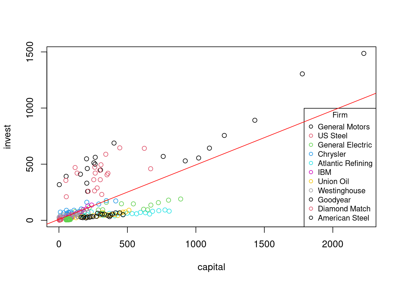
The observations appear in clusters, with each firm forming a cluster. This suggests potential problems with the pooled approach if we use classical standard errors.
The error covariance matrix for panel data has a block-diagonal structure: \boldsymbol D = \text{Var}[\boldsymbol u| \boldsymbol X] = \begin{pmatrix} \boldsymbol D_1 & \boldsymbol 0 & \ldots & \boldsymbol 0 \\ \boldsymbol 0 & \boldsymbol D_2 & \ldots & \boldsymbol 0 \\ \vdots & \vdots & \ddots & \vdots \\ \boldsymbol 0 & \boldsymbol 0 & \ldots & \boldsymbol D_n \end{pmatrix}
where \boldsymbol D_i is the T \times T covariance matrix for individual i: \boldsymbol D_i = \begin{pmatrix} E[u_{i,1}^2|\boldsymbol X] & E[u_{i,1}u_{i,2}|\boldsymbol X] & \ldots & E[u_{i,1}u_{i,T}|\boldsymbol X] \\ E[u_{i,2}u_{i,1}|\boldsymbol X] & E[u_{i,2}^2|\boldsymbol X] & \ldots & E[u_{i,2}u_{i,T}|\boldsymbol X] \\ \vdots & \vdots & \ddots & \vdots \\ E[u_{i,T}u_{i,1}|\boldsymbol X] & E[u_{i,T} u_{i,2}|\boldsymbol X] & \ldots & E[u_{i,T}^2|\boldsymbol X] \\ \end{pmatrix}
The variance of the pooled OLS estimator is: \text{Var}[\widehat{\boldsymbol \beta}_{\text{pool}} | \boldsymbol X] = (\boldsymbol X' \boldsymbol X)^{-1} (\boldsymbol X' \boldsymbol D \boldsymbol X) (\boldsymbol X' \boldsymbol X)^{-1}
The cluster-robust covariance matrix estimator is: \widehat{\boldsymbol V}_{\text{pool}} = (\boldsymbol X' \boldsymbol X)^{-1} \sum_{i=1}^n \bigg( \sum_{t=1}^T \boldsymbol X_{it} \widehat u_{it} \bigg) \bigg( \sum_{t=1}^T \boldsymbol X_{it} \widehat u_{it} \bigg)' (\boldsymbol X' \boldsymbol X)^{-1}
We can implement this using the fixest package:
# Pooled regression with fixest
fit_pool_fe = feols(invest ~ capital, data = Grunfeld)

# Incorrect Classical Standard Errors
summary(fit_pool_fe)
OLS estimation, Dep. Var.: invest
Observations: 220
Standard-errors: IID
Estimate Std. Error t value Pr(>|t|)
(Intercept) 8.565056 13.967368 0.613219 0.54037
capital 0.485191 0.035861 13.529645 < 2.2e-16 ***
---
Signif. codes: 0 '***' 0.001 '**' 0.01 '*' 0.05 '.' 0.1 ' ' 1
RMSE: 154.9 Adj. R2: 0.453935# Cluster-robust standard errors (clustered by firm)
summary(fit_pool_fe, cluster = "firm")OLS estimation, Dep. Var.: invest
Observations: 220
Standard-errors: Clustered (firm)
Estimate Std. Error t value Pr(>|t|)
(Intercept) 8.565056 25.729726 0.332886 0.7460942
capital 0.485191 0.132374 3.665310 0.0043507 **
---
Signif. codes: 0 '***' 0.001 '**' 0.01 '*' 0.05 '.' 0.1 ' ' 1
RMSE: 154.9 Adj. R2: 0.4539357.3 Time-invariant Regressors
Consider a simple panel regression model: Y_{it} = \beta_1 + \beta_2 X_{it} + \beta_3 Z_i + u_{it} \tag{7.1}
Here, Z_i represents a time-invariant variable specific to individual i (e.g., gender, ethnicity, birthplace).
With the usual exogeneity condition E[u_{it}|X_{it}, Z_i], the coefficient \beta_2 can be interpreted as the marginal effect of X_{it} on Y_{it}, holding Z_i constant.
The key advantage of panel data is that we can control for a time-invariant variable Z_i even if it is unobserved.
To see this, consider data from just two time periods, t=1 and t=2. Taking the difference between time periods: \begin{align*} Y_{i2} - Y_{i1} &= (\beta_1 + \beta_2 X_{i2} + \beta_3 Z_i + u_{i2}) - (\beta_1 + \beta_2 X_{i1} + \beta_3 Z_i + u_{i1}) \\ &= \beta_2(X_{i2} - X_{i1}) + (u_{i2} - u_{i1}) \end{align*}
This first-differencing transformation eliminates both the intercept \beta_1 and the effect of the time-invariant variable \beta_3 Z_i.
The coefficient \beta_2 is simply the regression coefficient from the first-differenced model: \Delta Y_{i} = \beta_2 \Delta X_{i} + \Delta u_{i}, where \Delta Y_{i} = Y_{i2} - Y_{i1}, \Delta X_{i} = X_{i2} - X_{i1}, and \Delta u_{i} = u_{i2} - u_{i1}.
Therefore, \beta_2 can be estimated from a regression of \Delta Y_i on \Delta X_i without intercept. We do not need to observe Z_i to estimate \beta_2 from model Equation 7.1.
We can combine the terms \beta_1 and \beta_3 Z_i into a single individual fixed effect \alpha_i = \beta_1 + \beta_3 Z_i. This term represents all unobserved, time-constant factors that affect the dependent variable.
7.4 The Fixed Effects Model
Let’s formalize the fixed effects model. Consider a panel dataset with dependent variable Y_{it}, a vector of k independent variables \boldsymbol X_{it}, and an unobserved individual fixed effect \alpha_i for i=1, \ldots, n and t=1, \ldots, T.
Fixed Effects Regression Model
The fixed effects regression model for individual i=1, \ldots, n and time t=1, \ldots, T is: Y_{it} = \alpha_i + \boldsymbol X_{it}'\boldsymbol \beta + u_{it} \tag{7.2} where \boldsymbol \beta = (\beta_1, \ldots, \beta_k)' is the k \times 1 vector of regression coefficients, \alpha_i is the individual fixed effect, and u_{it} is the error term.
Identification Assumptions
To identify \beta_j as the ceteris paribus marginal effect of X_{j,it} on Y_{it}, holding constant the fixed effect \alpha_i and the other regressors, we need to make some assumptions.
Strict exogeneity conditional on fixed effects: E[u_{it} | \boldsymbol{X}_{i1}, \ldots, \boldsymbol{X}_{iT}, \alpha_i] = 0 for all t. This means that the error u_{it} is uncorrelated with the regressors in all time periods, conditional on the fixed effect.
Time-varying regressors: There must be variation in \boldsymbol{X}_{j,it} over time within each individual. Time-invariant regressors are absorbed by the fixed effect \alpha_i and cannot be separately identified.
If strict exogeneity is violated (e.g., due to feedback effects where Y_{it} affects future values of \boldsymbol{X}_{is} for s > t), then the fixed effects estimator will be inconsistent. In this case, dynamic panel data models may be appropriate.
First-Differencing Estimator
As shown earlier, we can eliminate the fixed effects by taking first differences. Using \Delta Y_{it} = Y_{it} - Y_{i,t-1} as the dependent variable and inserting model Equation 7.2, we get: \Delta Y_{it} = (\Delta \boldsymbol X_{it})' \boldsymbol \beta + \Delta u_{it} \tag{7.3}
where \Delta \boldsymbol X_{it} = \boldsymbol X_{it} - \boldsymbol X_{i,t-1} and \Delta u_{it} = u_{it} - u_{i,t-1}.
We can then apply OLS to this transformed model:
# Create first differences manually for demonstration
diffcapital = c(aggregate(Grunfeld$capital, by = list(Grunfeld$firm), FUN = diff)$x)
diffinvest = c(aggregate(Grunfeld$inv, by = list(Grunfeld$firm), FUN = diff)$x)

# First-difference regression
lm(diffinvest ~ diffcapital - 1)
Call:
lm(formula = diffinvest ~ diffcapital - 1)

Coefficients:
diffcapital
     0.2307
A problem with this differenced estimator is that the transformed error term \Delta u_{it} defines an artificial correlation structure, which makes the estimator non-optimal. \Delta u_{i,t+1} = u_{i,t+1} - u_{i,t} is correlated with \Delta u_{i,t} = u_{i,t} - u_{i,t-1} through u_{i,t}.
Within Estimator
An efficient estimator can be obtained by a different transformation. The idea is to consider the individual specific means \overline Y_{i\cdot} = \frac{1}{T} \sum_{t=1}^T Y_{it}, \quad \overline{\boldsymbol X}_{i\cdot} = \frac{1}{T} \sum_{t=1}^T \boldsymbol X_{it}, \quad \overline{u}_{i\cdot} = \frac{1}{T} \sum_{t=1}^T u_{it}
Taking the means over t of both sides of Equation 7.2 implies \overline{Y}_{i\cdot} = \alpha_i + \overline{\boldsymbol X}_{i\cdot}'\boldsymbol \beta + \overline{u}_{i\cdot}. \tag{7.4}
Then, we subtract these means from the original equation: Y_{it} - \overline Y_{i\cdot} = (\boldsymbol X_{it} - \overline{\boldsymbol X}_{i\cdot})'\boldsymbol \beta + (u_{it} - \overline{u}_{i\cdot}) The fixed effect \alpha_i drops out.
The deviations from the individual specific means are called within transformations: \dot Y_{it} = Y_{it} - \overline Y_{i\cdot}, \quad \dot{\boldsymbol X}_{it} = \boldsymbol X_{it} - \overline{\boldsymbol X}_{i\cdot}, \quad \dot u_{it} = u_{it} - \overline{u}_{i\cdot} The within-transfromed model equation is \dot Y_{it} = \dot{\boldsymbol X}_{it}'\boldsymbol \beta + \dot u_{it} \tag{7.5}
The within estimator (also called the fixed effects estimator) is: \widehat{\boldsymbol \beta}_{\text{fe}} = \bigg( \sum_{i=1}^n \sum_{t=1}^T \dot{\boldsymbol X}_{it} \dot{\boldsymbol X}_{it}' \bigg)^{-1} \bigg( \sum_{i=1}^n \sum_{t=1}^T \dot{\boldsymbol X}_{it} \dot Y_{it} \bigg)
# Fixed effects estimation using fixest
fit_fe = feols(invest ~ capital, fixef = "firm", data = Grunfeld)
fit_fe$coefficients
capital
0.3707023 Fixed Effects Regression Assumptions
(A1-fe) E[u_{it} | \boldsymbol X_{i1}, \ldots, \boldsymbol X_{iT}, \alpha_i] = 0.
(A2-fe) (\alpha_i, Y_{i1}, \ldots, Y_{iT}, \boldsymbol X_{i1}', \ldots, \boldsymbol X_{iT}')_{i=1}^n is an i.i.d. sample.
(A3-fe) kur(Y_{it}) < \infty, kur(u_{it}) < \infty.
(A4-fe) \sum_{i=1}^n \sum_{t=1}^T \dot{\boldsymbol X}_{it} \dot{\boldsymbol X}_{it}' is invertible.
(A1-fe) is the same as (A1-pool), but now we condition on the unobserved fixed effect \alpha_i.
(A2-fe) is a standard random sampling assumption indicating that individuals i=1, \ldots, n are randomly sampled.
(A3-fe) ensures finite fourth moments, which is a requirement for asymptotic normality of the estimator.
(A4-fe) is satisfied if there is no perfect multicollinearity and if no regressor is constant over time for any individual.
Under (A2-fe), the collection of the within-transformed variables of individual i, (\dot Y_{i1}, \ldots, \dot Y_{iT}, \dot{\boldsymbol X}_{i1}, \ldots, \dot{\boldsymbol X}_{iT}, \dot u_{i1}, \ldots, \dot u_{iT}), forms an i.i.d. sequence for i=1, \ldots, n.
The within-transformed variables satisfy (A1-pool)–(A4-pool), which mean that its asymptotic distribution is: \sqrt{n}(\widehat{\boldsymbol \beta}_{\text{fe}} - \boldsymbol \beta) \xrightarrow{d} N(0, \boldsymbol W^{-1} \boldsymbol \Psi \boldsymbol W^{-1}), \qquad \text{as } n \to \infty,
where \boldsymbol W = E(\frac{1}{T}\sum_{t=1}^T \dot{\boldsymbol X}_{it} \dot{\boldsymbol X}_{it}') and \boldsymbol \Psi = E((\frac{1}{T}\sum_{t=1}^T \dot{\boldsymbol X}_{it} \dot{u}_{it})(\frac{1}{T}\sum_{t=1}^T \dot{\boldsymbol X}_{it} \dot{u}_{it})').
Hence, we can apply the cluster-robust covariance matrix estimator of the pooled regression to the within-transformed variables:
# Inference with cluster-robust standard errors
summary(fit_fe, cluster = "firm")
OLS estimation, Dep. Var.: invest
Observations: 220
Fixed-effects: firm: 11
Standard-errors: Clustered (firm)
Estimate Std. Error t value Pr(>|t|)
capital 0.370702 0.064785 5.72203 0.0001924 ***
---
Signif. codes: 0 '***' 0.001 '**' 0.01 '*' 0.05 '.' 0.1 ' ' 1
RMSE: 58.9 Adj. R2: 0.91717
Within R2: 0.659603Dummy Variable Approach
An equivalent way to estimate the fixed effects model is to include a dummy variable for each individual. This approach is known as the least squares dummy variable (LSDV) estimator:
# Equivalent to fit_fe
fit_fe_lsdv = lm(invest ~ capital + factor(firm) - 1, data = Grunfeld)
fit_fe_lsdv$coefficients
capital factor(firm)General Motors
0.3707023 367.6436372
factor(firm)US Steel factor(firm)General Electric
301.1715657 -46.0502428
factor(firm)Chrysler factor(firm)Atlantic Refining
41.1776965 -118.6424177
factor(firm)IBM factor(firm)Union Oil
16.7523079 -69.1553441
factor(firm)Westinghouse factor(firm)Goodyear
11.1445528 -68.5432229
factor(firm)Diamond Match factor(firm)American Steel
0.8819721 -18.3676804 The coefficient on the regressor capital is the same as in the within estimator. However, the LSDV approach becomes computationally intensive with many individuals, and the standard errors need to be adjusted for clustering.
7.5 Time Fixed Effects
While individual fixed effects control for unobserved heterogeneity across individuals, we might also want to control for factors that vary over time but are constant across individuals (e.g., macroeconomic conditions, policy changes).
The time fixed effects model is: Y_{it} = \lambda_t + \boldsymbol X_{it}' \boldsymbol \beta + u_{it} \tag{7.6}
where \lambda_t captures time-specific effects. Similar to individual fixed effects, we can rewrite this model by demeaning across time: Y_{it} - \overline Y_{\cdot t} = (\boldsymbol X_{it} - \overline{\boldsymbol X}_{\cdot t})' \boldsymbol \beta + (u_{it} - \overline{u}_{\cdot t})
where the time-specific means are: \overline Y_{\cdot t} = \frac{1}{n} \sum_{i=1}^n Y_{it}, \quad \overline{\boldsymbol X}_{\cdot t} = \frac{1}{n} \sum_{i=1}^n \boldsymbol X_{it}, \quad \overline{u}_{\cdot t} = \frac{1}{n} \sum_{i=1}^n u_{it}.
Hence, we regress Y_{it} - \overline Y_{\cdot t} on \boldsymbol X_{it} - \overline{\boldsymbol X}_{\cdot t} to estimate \boldsymbol \beta in Equation 7.6.
# Time fixed effects
fit_timefe = feols(invest ~ capital, fixef = "year", data = Grunfeld)
summary(fit_timefe, cluster = "firm")
OLS estimation, Dep. Var.: invest
Observations: 220
Fixed-effects: year: 20
Standard-errors: Clustered (firm)
Estimate Std. Error t value Pr(>|t|)
capital 0.539676 0.163321 3.30438 0.0079544 **
---
Signif. codes: 0 '***' 0.001 '**' 0.01 '*' 0.05 '.' 0.1 ' ' 1
RMSE: 151.1 Adj. R2: 0.430515
Within R2: 0.4501157.6 Two-way Fixed Effects
We can combine both individual and time fixed effects in a two-way fixed effects model: Y_{it} = \alpha_i + \lambda_t + \boldsymbol X_{it}' \boldsymbol \beta + u_{it} \tag{7.7}
This model controls for both individual-specific and time-specific unobserved factors. To estimate it, we apply a two-way transformation that subtracts individual means, time means, and adds back the overall mean: \ddot Y_{it} = Y_{it} - \overline Y_{i \cdot} - \overline Y_{\cdot t} + \overline Y \ddot{\boldsymbol X}_{it} = {\boldsymbol X}_{it} - \overline{\boldsymbol X}_{i \cdot} - \overline{\boldsymbol X}_{\cdot t} + \overline{\boldsymbol X}
To see why this is useful, consider the following transformations applied to the left-hand side of Equation 7.7:
- Individual specific mean: \overline Y_{i \cdot} = \alpha_i + \overline \lambda + \overline{\boldsymbol X}_{i\cdot}'\boldsymbol \beta + \overline u_{i\cdot}, where \overline \lambda = \frac{1}{T} \sum_{t=1}^T \lambda_t.
- Time specific mean: \overline Y_{\cdot t} = \overline \alpha + \lambda_t + \overline{\boldsymbol X}_{\cdot t}'\boldsymbol \beta + \overline u_{\cdot t}, where \overline \alpha = \frac{1}{n} \sum_{i=1}^n \alpha_i.
- Total mean: \overline Y = \frac{1}{nT} \sum_{i=1}^n \sum_{t=1}^T Y_{it} = \overline \alpha + \overline \lambda + \overline{\boldsymbol X}'\boldsymbol \beta + \overline u, where \overline{\boldsymbol X} = \frac{1}{nT} \sum_{i=1}^n \sum_{t=1}^T \boldsymbol X_{it} and \overline u = \frac{1}{nT} \sum_{i=1}^n \sum_{t=1}^T u_{it}.
The transformed model is: \ddot Y_{it} = \ddot{\boldsymbol X}_{it}'\boldsymbol \beta + \ddot u_{it} \tag{7.8} where \ddot u_{it} = u_{it} - \overline u_{i \cdot} - \overline u_{\cdot t} + \overline u.
Hence, we estimate \boldsymbol \beta by regressing \ddot Y_{it} on \ddot{\boldsymbol X}_{it}.
# Two-way fixed effects
fit_2wayfe = feols(invest ~ capital, fixef = c("firm", "year"), data = Grunfeld)
summary(fit_2wayfe, cluster = "firm")
OLS estimation, Dep. Var.: invest
Observations: 220
Fixed-effects: firm: 11, year: 20
Standard-errors: Clustered (firm)
Estimate Std. Error t value Pr(>|t|)
capital 0.40875 0.062522 6.53767 6.5744e-05 ***
---
Signif. codes: 0 '***' 0.001 '**' 0.01 '*' 0.05 '.' 0.1 ' ' 1
RMSE: 54.7 Adj. R2: 0.921459
Within R2: 0.60632 For inference, we use cluster-robust standard errors:
# Cluster-robust standard errors
summary(fit_2wayfe, cluster = "firm")
OLS estimation, Dep. Var.: invest
Observations: 220
Fixed-effects: firm: 11, year: 20
Standard-errors: Clustered (firm)
Estimate Std. Error t value Pr(>|t|)
capital 0.40875 0.062522 6.53767 6.5744e-05 ***
---
Signif. codes: 0 '***' 0.001 '**' 0.01 '*' 0.05 '.' 0.1 ' ' 1
RMSE: 54.7 Adj. R2: 0.921459
Within R2: 0.60632 7.7 Comparison of Panel Models
Let’s compare the different panel regression approaches:
# Create a list of models
models = list(
  "OLS-IID" = feols(invest ~ capital, data = Grunfeld),
  "OLS-CL" = feols(invest ~ capital, data = Grunfeld, cluster = "firm"),
  "FE" = feols(invest ~ capital, fixef = "firm", data = Grunfeld, cluster = "firm"),
  "Time FE" = feols(invest ~ capital, fixef = "year", data = Grunfeld, cluster = "firm"),
  "Two-way FE" = feols(invest ~ capital, fixef = c("firm", "year"), data = Grunfeld, cluster = "firm")
)

# Generate the comparison table with clustered standard errors
modelsummary(models, stars = TRUE)| OLS-IID | OLS-CL | FE | Time FE | Two-way FE | |
|---|---|---|---|---|---|
| + p | |||||
| (Intercept) | 8.565 | 8.565 | |||
| (13.967) | (25.730) | ||||
| capital | 0.485*** | 0.485** | 0.371*** | 0.540** | 0.409*** |
| (0.036) | (0.132) | (0.065) | (0.163) | (0.063) | |
| Num.Obs. | 220 | 220 | 220 | 220 | 220 |
| R2 | 0.456 | 0.456 | 0.921 | 0.483 | 0.932 |
| R2 Adj. | 0.454 | 0.454 | 0.917 | 0.431 | 0.921 |
| R2 Within | 0.660 | 0.450 | 0.606 | ||
| R2 Within Adj. | 0.658 | 0.447 | 0.604 | ||
| AIC | 2847.2 | 2847.2 | 2441.9 | 2874.4 | 2447.2 |
| BIC | 2854.0 | 2854.0 | 2482.7 | 2945.6 | 2552.4 |
| RMSE | 154.91 | 154.91 | 58.93 | 151.14 | 54.70 |
| Std.Errors | IID | by: firm | by: firm | by: firm | by: firm |
| FE: firm | X | X | |||
| FE: year | X | X | |||
7.8 Panel R-squared
In panel data models with fixed effects, two different R-squared measures provide distinct information about model fit:
Within R-squared
The within R-squared measures the proportion of within-individual variation explained by the model. For the three different fixed effects specifications, the within R-squared is defined as follows:
- For individual fixed effects: R^2_{wit} = 1 - \frac{\sum_{i=1}^n \sum_{t=1}^T (\dot{Y}_{it} - \dot{\boldsymbol{X}}_{it}'\hat{\boldsymbol{\beta}})^2}{\sum_{i=1}^n \sum_{t=1}^T \dot{Y}_{it}^2}
- For time fixed effects: R^2_{wit} = 1 - \frac{\sum_{i=1}^n \sum_{t=1}^T (Y_{it} - \overline{Y}_{\cdot t} - ({\boldsymbol{X}}_{it} - \overline{\boldsymbol{X}}_{\cdot t})'\hat{\boldsymbol{\beta}})^2}{\sum_{i=1}^n \sum_{t=1}^T (Y_{it} - \overline{Y}_{\cdot t})^2}
- For two-way fixed effects: R^2_{wit} = 1 - \frac{\sum_{i=1}^n \sum_{t=1}^T (\ddot{Y}_{it} - \ddot{\boldsymbol{X}}_{it}'\hat{\boldsymbol{\beta}})^2}{\sum_{i=1}^n \sum_{t=1}^T \ddot{Y}_{it}^2}
In the panel models for the Grunfeld data, the individual fixed effects model has the highest within R-squared (0.660), suggesting that within-firm variations in capital explain 66% of within-firm variations in investment.
This drops to 0.450 in the time fixed effects model, indicating that year-specific factors share substantial variation with capital stock within each year.
The higher within R-squared for individual fixed effects (0.660) compared to time fixed effects (0.450) suggests that firm-specific characteristics play a greater role in explaining variation in investment than year-specific factors.
The two-way fixed effects model shows an intermediate within R-squared (0.606). This model controls for more confounding factors from both dimensions, resulting in an estimate that is likely closer to the true causal effect of capital on investment, though with somewhat reduced statistical power.
Overall R-squared
The overall R-squared measures how well the complete model (including fixed effects) explains the total variation:
R^2_{ov} = 1 - \frac{\sum_{i=1}^n \sum_{t=1}^T (Y_{it} - \hat{Y}_{it})^2}{\sum_{i=1}^n \sum_{t=1}^T (Y_{it} - \overline{Y})^2} Here, \hat{Y}_{it} is the fitted value of the corresponding model.
The overall R-squared values reveal how different specifications explain investment variation: pooled OLS (45.6%), firm fixed effects (92.1%), time fixed effects (48.3%), and two-way fixed effects (93.2%). The large jump when adding firm fixed effects, compared to the minimal improvement from time fixed effects, confirms that firm-specific characteristics are far more important determinants of investment behavior than year-specific factors.
The within R-squared is typically more relevant because it isolates the relationship of interest after controlling for unobserved heterogeneity. However, if you’re interested in overall predictive power, the overall R-squared provides that information.
Fitted Values
The overall R-squared requires the computation of the fitted values \hat{Y}_{it}. To compute them, we require some estimates or averages of the fixed effects themselves.
- For individual fixed effects: \begin{align*} \hat{Y}_{it} &= \hat{\alpha}_i + \boldsymbol{X}_{it}'\hat{\boldsymbol{\beta}} \\ \hat{\alpha}_i &= \overline{Y}_{i\cdot} - \overline{\boldsymbol{X}}_{i\cdot}'\hat{\boldsymbol{\beta}} \end{align*}
- For time fixed effects: \begin{align*} \hat{Y}_{it} &= \hat{\lambda}_t + \boldsymbol{X}_{it}'\hat{\boldsymbol{\beta}} \\ \hat{\lambda}_t &= \overline{Y}_{\cdot t} - \overline{\boldsymbol{X}}_{\cdot t}'\hat{\boldsymbol{\beta}} \end{align*}
- For two-way fixed effects: \hat{Y}_{it} = \hat{\alpha}_i + \hat{\lambda}_t - \hat{\mu} + \boldsymbol{X}_{it}'\hat{\boldsymbol{\beta}}, where \begin{align*} \hat{\alpha}_i &= \overline{Y}_{i\cdot} - \overline{\boldsymbol{X}}_{i\cdot}'\hat{\boldsymbol{\beta}} - \hat{\mu} \\ \hat{\lambda}_t &= \overline{Y}_{\cdot t} - \overline{\boldsymbol{X}}_{\cdot t}'\hat{\boldsymbol{\beta}} - \hat{\mu} \\ \hat{\mu} &= \overline{Y} - \overline{\boldsymbol{X}}'\hat{\boldsymbol{\beta}} \end{align*}
While these fixed effects estimates are useful for calculating fitted values, they are not recommended for direct interpretation. Fixed effects capture all time-invariant (or unit-invariant) factors, observed and unobserved, making them a “black box” rather than specific causal parameters.
7.9 Application: Traffic Fatalities
To illustrate the importance of fixed effects in empirical work, let’s examine how government policies affect traffic fatalities. We’ll use the Fatalities dataset from the AER package, which contains panel data on traffic fatalities, drunk driving laws, and beer taxes for U.S. states from 1982 to 1988.
data(Fatalities, package = "AER")
# Create the fatality rate per 10,000 population
Fatalities$fatal_rate = Fatalities$fatal / Fatalities$pop * 10000
Cross-sectional Analysis
First, let’s examine the relationship between beer taxes and traffic fatality rates using pooled OLS:
OLS estimation, Dep. Var.: fatal_rate
Observations: 336
Standard-errors: Clustered (state)
            Estimate Std. Error  t value  Pr(>|t|)
(Intercept) 1.853308   0.118519 15.63719 < 2.2e-16 ***
beertax     0.364605   0.119686  3.04636 0.0037916 **
---
Signif. codes:  0 '***' 0.001 '**' 0.01 '*' 0.05 '.' 0.1 ' ' 1
RMSE: 0.542116   Adj. R2: 0.090648
Surprisingly, we find a positive relationship between beer taxes and fatality rates. This counterintuitive result likely stems from omitted variable bias.
Fixed Effects Approach
Now, let’s use the panel structure to control for unobserved state-specific factors:
# State fixed effects model
fatal_fe = feols(fatal_rate ~ beertax, fixef = "state", data = Fatalities, cluster = "state")
summary(fatal_fe)
OLS estimation, Dep. Var.: fatal_rate
Observations: 336
Fixed-effects: state: 48
Standard-errors: Clustered (state)
Estimate Std. Error t value Pr(>|t|)
beertax -0.655874 0.291856 -2.24725 0.029358 *
---
Signif. codes: 0 '***' 0.001 '**' 0.01 '*' 0.05 '.' 0.1 ' ' 1
RMSE: 0.17547 Adj. R2: 0.889129
Within R2: 0.040745With state fixed effects, the coefficient becomes negative, aligning with our theoretical expectation that higher beer taxes should reduce drunk driving and fatalities.
Let’s add time fixed effects
# State fixed effects model
fatal_twoway = feols(fatal_rate ~ beertax, fixef = c("state", "year"), data = Fatalities, cluster = "state")
summary(fatal_twoway)
OLS estimation, Dep. Var.: fatal_rate
Observations: 336
Fixed-effects: state: 48, year: 7
Standard-errors: Clustered (state)
Estimate Std. Error t value Pr(>|t|)
beertax -0.63998 0.357078 -1.79227 0.079528 .
---
Signif. codes: 0 '***' 0.001 '**' 0.01 '*' 0.05 '.' 0.1 ' ' 1
RMSE: 0.171819 Adj. R2: 0.891425
Within R2: 0.036065Finally, let’s add control variables that are neither constant over time nor across states:
Fatalities$punish = ifelse(Fatalities$jail == "yes" | Fatalities$service == "yes",
                           "yes", "no")
fatal_full = feols(fatal_rate ~ beertax + drinkage + punish + miles + unemp + log(income), fixef = c("state", "year"),
                   data = Fatalities, cluster = "state")
NOTE: 1 observation removed because of NA values (RHS: 1).summary(fatal_full)OLS estimation, Dep. Var.: fatal_rate
Observations: 335
Fixed-effects: state: 48, year: 7
Standard-errors: Clustered (state)
Estimate Std. Error t value Pr(>|t|)
beertax -0.45646674 0.30680756 -1.487795 0.14348400
drinkage -0.00215674 0.02151945 -0.100223 0.92059358
punishyes 0.03898148 0.10316089 0.377871 0.70722783
miles 0.00000898 0.00000710 1.265052 0.21208923
unemp -0.06269441 0.01322938 -4.739031 0.00002021 ***
log(income) 1.78643540 0.64339251 2.776587 0.00786399 **
---
Signif. codes: 0 '***' 0.001 '**' 0.01 '*' 0.05 '.' 0.1 ' ' 1
RMSE: 0.140556 Adj. R2: 0.926185
Within R2: 0.356781This comprehensive model still produces a negative coefficient, though effect becomes insignificant with the addition of control variables.
# Create model list
fatal_models = list(
  fatal_cs,
  fatal_fe,
  fatal_twoway,
  fatal_full
)
# Generate comparison table
modelsummary(fatal_models, stars = TRUE)| (1) | (2) | (3) | (4) | |
|---|---|---|---|---|
| + p | ||||
| (Intercept) | 1.853*** | |||
| (0.119) | ||||
| beertax | 0.365** | -0.656* | -0.640+ | -0.456 |
| (0.120) | (0.292) | (0.357) | (0.307) | |
| drinkage | -0.002 | |||
| (0.022) | ||||
| punishyes | 0.039 | |||
| (0.103) | ||||
| miles | 0.000 | |||
| (0.000) | ||||
| unemp | -0.063*** | |||
| (0.013) | ||||
| log(income) | 1.786** | |||
| (0.643) | ||||
| Num.Obs. | 336 | 336 | 336 | 335 |
| R2 | 0.093 | 0.905 | 0.909 | 0.939 |
| R2 Adj. | 0.091 | 0.889 | 0.891 | 0.926 |
| R2 Within | 0.041 | 0.036 | 0.357 | |
| R2 Within Adj. | 0.037 | 0.033 | 0.343 | |
| AIC | 546.1 | -117.9 | -120.1 | -243.9 |
| BIC | 553.7 | 69.1 | 89.9 | -15.1 |
| RMSE | 0.54 | 0.18 | 0.17 | 0.14 |
| Std.Errors | by: state | by: state | by: state | by: state |
| FE: state | X | X | X | |
| FE: year | X | X | ||
The changing sign of the beertax coefficient across specifications illustrates the importance of controlling for unobserved heterogeneity in panel data:
In the pooled model, the positive coefficient might reflect that states with higher fatality rates tend to implement higher beer taxes as a policy response.
Once we control for state fixed effects, we isolate the within-state variation and find the expected negative relationship: when a state raises its beer tax, fatality rates decrease.
Adding year fixed effects accounts for national trends in fatality rates, such as changes in vehicle safety technology or nationwide campaigns against drunk driving.
In the full model with additional controls, the beer tax coefficient remains negative but loses statistical significance. This suggests that its effect may be partially captured by other policy variables or that we lack statistical power to precisely estimate the effect when including multiple controls.