cps = read.csv("cps.csv")
exper = cps$experience
wage = cps$wage
edu = cps$education
fem = cps$female2 Summary Statistics
In statistics, a univariate dataset Y_1, \ldots, Y_n or a multivariate dataset \boldsymbol X_1, \ldots, \boldsymbol X_n is often called a sample. It typically represents observations collected from a larger population. The sample distribution indicates how the sample values are distributed across possible outcomes.
Summary statistics, such as the sample mean and sample variance, provide a concise representation of key characteristics of the sample distribution. These summary statistics are related to the sample moments of a dataset.
2.1 Sample moments
The r-th sample moment about the origin (also called the r-th raw moment) is defined as \overline{Y^r} = \frac{1}{n} \sum_{i=1}^n Y_i^r.
Mean
For example, the first sample moment (r=1) is the sample mean (arithmetic mean): \overline Y = \frac{1}{n} \sum_{i=1}^n Y_i.
The sample mean is the most common measure of central tendency. In i.i.d. samples, it converges in probability to the expected value as sample size grows (law of large numbers). This makes it a consistent estimator for the population mean: \overline Y \overset{p}{\rightarrow} \mu = E[Y] \quad \text{as} \ n \to \infty.
To compute the sample mean of a vector Y in R, use mean(Y) or alternatively sum(Y)/length(Y). The r-th sample moment can be calculated with mean(Y^r).
2.2 Central sample moments
The r-th central sample moment is the average of the r-th powers of the deviations from the sample mean: \frac{1}{n} \sum_{i=1}^n (Y_i - \overline Y)^r
Variance
For example, the second central moment (r=2) is the sample variance: \widehat \sigma_Y^2 = \frac{1}{n} \sum_{i=1}^n (Y_i - \overline Y)^2 = \overline{Y^2} - \overline Y^2.
The sample variance measures the spread or dispersion of the data around the sample mean. It is a consistent estimator for the population variance \sigma^2 = Var(Y) = E[(Y - E[Y])^2] = E[Y^2] - E[Y]^2 if the sample is i.i.d.
Standard Deviation
The sample standard deviation is the square root of the sample variance: \widehat \sigma_Y = \sqrt{\widehat \sigma_Y^2} = \sqrt{\frac{1}{n} \sum_{i=1}^n (Y_i - \overline Y)^2} = \sqrt{\overline{Y^2} - \overline Y^2}
It quantifies the typical deviation of data points from the sample mean in the original units of measurement. It is a consistent estimator for the population standard deviation sd(Y) = \sqrt{Var(Y)}.
2.3 Adjustments
Degrees of Freedom
When computing the sample mean \overline Y, we have n degrees of freedom because all data points Y_1, \ldots, Y_n can vary freely.
When computing variances, we take the sample mean of the squared deviations (Y_1 - \overline Y)^2, \ldots, (Y_n - \overline Y)^2. These elements cannot vary freely because \overline Y is computed from the same sample and implies the constraint \frac{1}{n} \sum_{i=1}^n (Y_i - \overline{Y}) = 0.
This means that the deviations are connected by this equation and are not all free to vary. Knowing the first n-1 of the deviations determines the last one: (Y_n - \overline Y) = - \sum_{i=1}^{n-1} (Y_i - \overline Y). Therefore, only n-1 deviations can vary freely, which results in n-1 degrees of freedom for the sample variance.
Adjusted Sample Variance
Because \sum_{i=1}^{n} (Y_i - \overline Y)^2 effectively contains only n-1 freely varying summands, it is common to account for this fact. The adjusted sample variance uses n−1 in the denominator: s_Y^2 = \frac{1}{n-1} \sum_{i=1}^n (Y_i - \overline Y)^2. The adjusted sample variance relates to the unadjusted sample variance as: s_Y^2 = \frac{n}{n-1} \widehat \sigma_Y^2. The adjusted sample standard deviation is: s_Y = \sqrt{\frac{1}{n-1} \sum_{i=1}^n (Y_i - \overline Y)^2} = \sqrt{\frac{n}{n-1}} \widehat \sigma_Y.
To compute the sample variance and sample standard deviation of a vector Y in R, use mean(Y^2)-mean(Y)^2 and sqrt(mean(Y^2)-mean(Y)^2), respectively. The built-in functions var(Y) and sd(Y) compute their adjusted versions.
Let’s compute the sample means, sample variances, and adjusted sample variances of some variables from the cps dataset.
[1] 22.2071065 23.9026619 13.9246187 0.4257223## Sample variance
c(mean(exper^2)- mean(exper)^2, mean(wage^2) - mean(wage)^2,
mean(edu^2) - mean(edu)^2, mean(fem^2) - mean(fem)^2)[1] 136.1098206 428.9398785 7.5318408 0.2444828[1] 136.1125031 428.9483320 7.5319892 0.2444876While the unadjusted version (using n in the denominator) yields a lower variance, it remains biased in finite samples. In contrast, the adjusted version (using n-1) eliminates this bias at the expense of slightly higher variance, illustrating a bias–variance tradeoff. In large samples, however, the difference becomes negligible and both estimators yield practically the same results.
2.4 Density estimation
A continuous random variable Y is characterized by a continuously differentiable CDF F(a) = P(Y \leq a). The derivative is known as the probability density function (PDF), defined as f(a) = F'(a). There are several methods to estimate this density function from sample data.
Histogram
Histograms offer an intuitive visual representation of the sample distribution of a variable. A histogram divides the data range into B bins, each of equal width h, and counts the number of observations n_j within each bin. The height of the histogram at a in the j-th bin is \widehat f(a) = \frac{n_j}{nh}. The histogram is the plot of these heights, displayed as rectangles, with their area normalized so that the total area equals 1.
par(mfrow = c(2,2))
hist(exper, probability = TRUE)
hist(wage, probability = TRUE)
hist(edu, probability = TRUE)
hist(fem, probability = TRUE)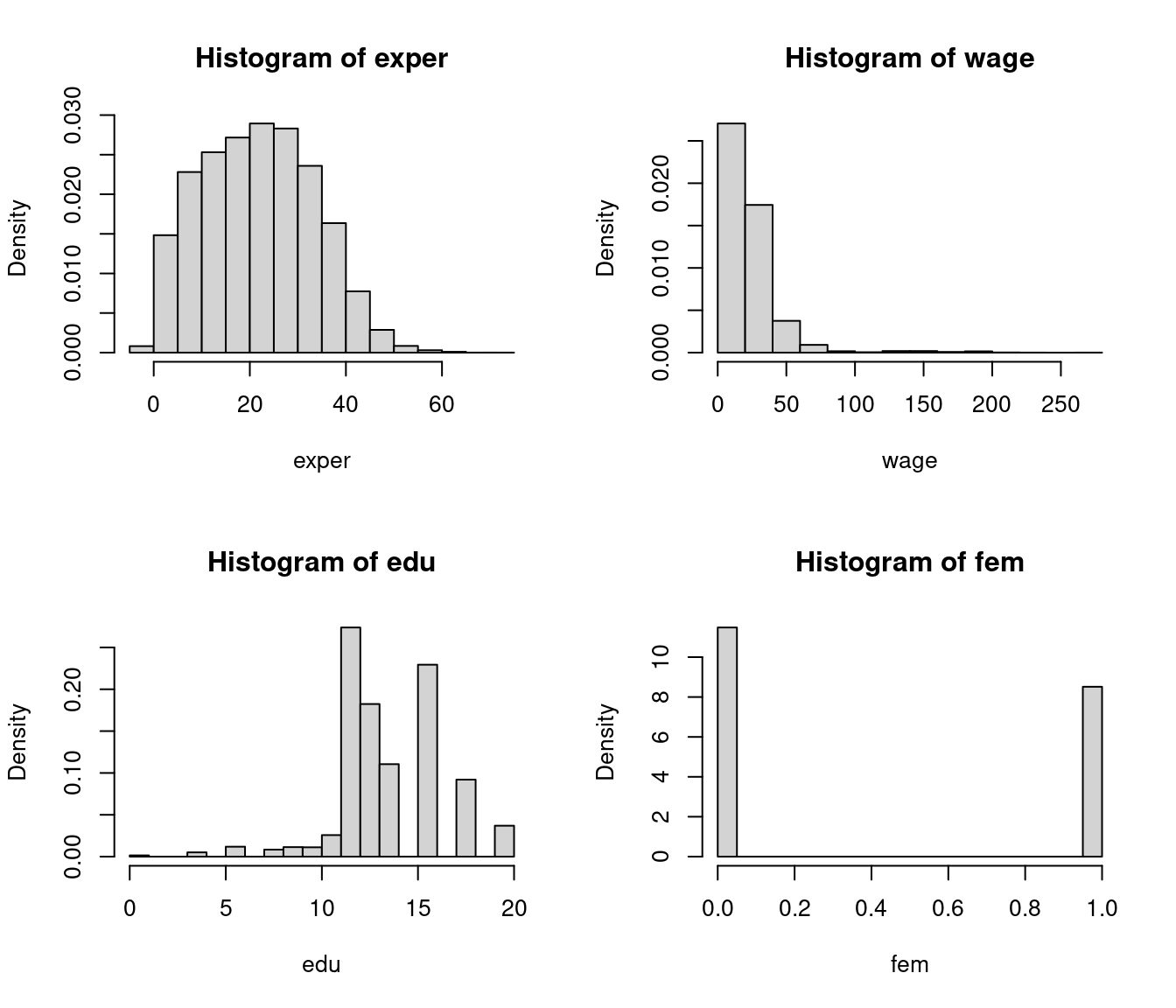
Running hist(wage, probability=TRUE) automatically selects a suitable number of bins B. Note that hist(wage) will plot absolute frequencies instead of relative ones. The shape of a histogram depends on the choice of B. You can experiment with different values using the breaks option:

Kernel density estimator
Suppose we want to estimate the wage density at a = 22 and consider the histogram density estimate with h=10. It is based on the frequency of observations in the interval [20, 30) which is a skewed window about a = 22.
It seems more sensible to center the window at 22, for example [17, 27) instead of [20, 30). It also seems sensible to give more weight to observations close to 22 and less to those at the edge of the window.
This idea leads to the kernel density estimator of f(a), which is a smooth version of the histogram:
\widehat f(a) = \frac{1}{nh} \sum_{i=1}^n K\Big(\frac{X_i - a}{h} \Big). Here, K(u) represents a weighting function known as a kernel function, and h > 0 is the bandwidth. A common choice for K(u) is the Gaussian kernel: K(u) = \phi(u) = \frac{1}{\sqrt{2 \pi}} \exp(-u^2/2).
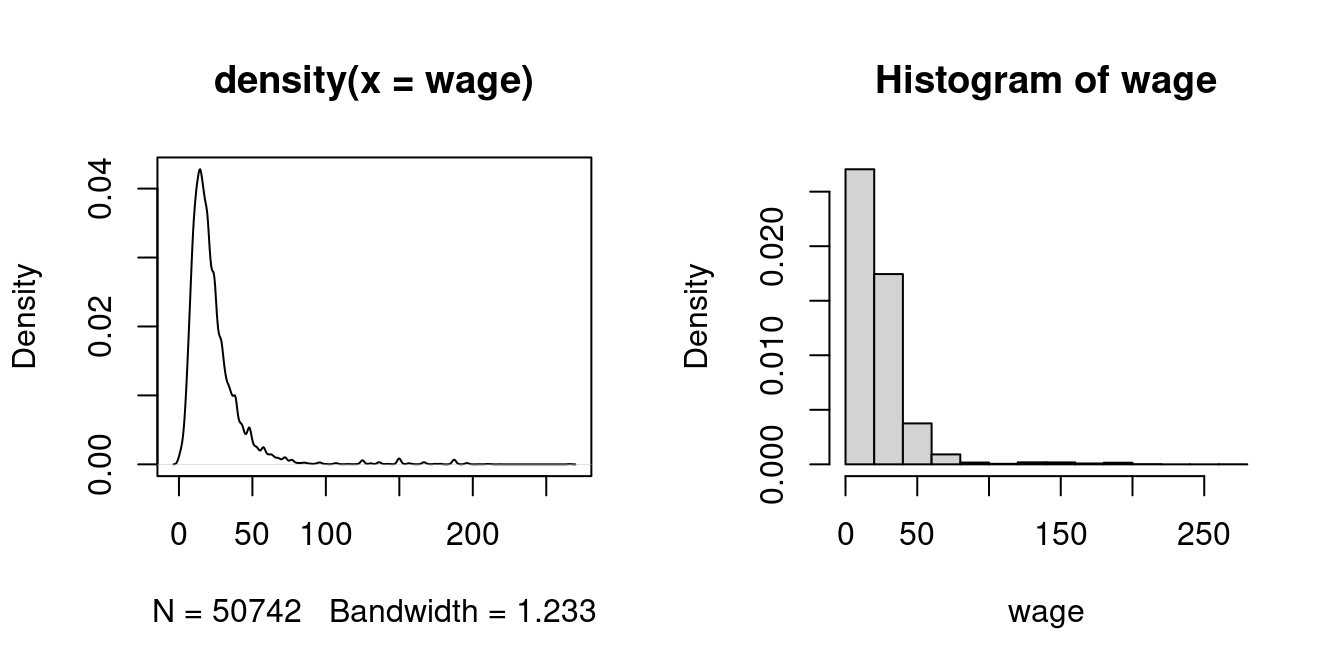
The density() function in R automatically selects an optimal bandwidth, but it also allows for manual bandwidth specification via density(wage, bw = your_bandwidth).
2.5 Higher Moments
The r-th standardized sample moment is the central moment normalized by the sample standard deviation raised to the power of r. It is defined as: \frac{1}{n} \sum_{i=1}^n \bigg(\frac{Y_i - \overline Y}{\widehat \sigma_Y}\bigg)^r
Skewness
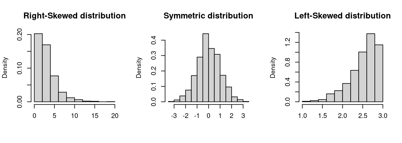
For example, the third standardized sample moment (r=3) is the sample skewness: \widehat{\text{ske}}(Y) = \frac{1}{n \widehat \sigma_Y^3} \sum_{i=1}^n (Y_i - \overline Y)^3. The skewness is a measure of asymmetry around the mean. A positive skewness indicates that the distribution has a longer or heavier tail on the right side (right-skewed), while a negative skewness indicates a longer or heavier tail on the left side (left-skewed). A perfectly symmetric distribution, such as the normal distribution, has a skewness of 0.
For i.i.d. samples, the sample skewness is a consistent estimator for the population skewness ske(Y) = \frac{E[(Y - E[Y])^3]}{sd(Y)^3}.
To compute the sample skewness in R, use:
For convenience, you can use the skewness(Y) function from the moments package, which performs the same calculation.
[1] 0.1862605 4.3201570 -0.2253251 0.3004446Wages are right-skewed because a few very rich individuals earn much more than the many with low to medium incomes. The other variables do not indicate any pronounced skewness.
Kurtosis
The sample kurtosis is the fourth standardized sample moment (r=4), commonly denoted as g_2: \widehat{\text{kur}}(Y) = \frac{1}{n \widehat \sigma_Y^4} \sum_{i=1}^n (Y_i - \overline Y)^4.
Kurtosis measures the “tailedness” or heaviness of the tails of a distribution and can indicate the presence of extreme outliers. The reference value of kurtosis is 3, which corresponds to the kurtosis of a normal distribution. Values greater than 3 suggest heavier tails, while values less than 3 indicate lighter tails.
For i.i.d. samples, the sample kurtosis is a consistent estimator for the population kurtosis kur(Y) = \frac{E[(Y - E[Y])^4]}{Var(Y)^2}.
To compute the sample kurtosis in R, use:
For convenience, you can use the kurtosis(Y) function from the moments package, which performs the same calculation.
[1] 2.374758 30.370331 4.498264 1.090267The variable wage exhibits heavy tails due to a few super-rich outliers in the sample. In contrast, fem has light tails because there are approximately equal numbers of women and men.
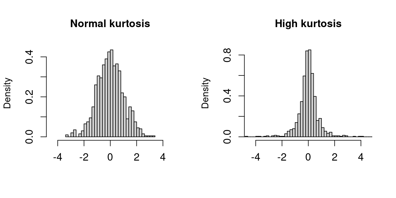
The plots display histograms of two standardized datasets (both have a sample mean of 0 and a sample variance of 1). The left dataset has a normal sample kurtosis (around 3), while the right dataset has a high sample kurtosis with heavier tails.
Kurtosis not only measures the heaviness of a distribution’s tails but also its peakedness. A high kurtosis indicates that data are more concentrated around the mean and in the extremes, meaning that extreme values occur more frequently than they would in a normal distribution.
In contrast, a low kurtosis signifies a flatter peak with lighter tails, suggesting fewer extreme observations. In finance and risk management, these differences are crucial because they affect the probability of rare but impactful events.
Some statistical software reports the excess kurtosis, which is defined as \widehat{kur} - 3. This shifts the reference value to 0 (instead of 3), making it easier to interpret: positive values indicate heavier tails than the normal distribution, while negative values indicate lighter tails. For example, the normal distribution has an excess kurtosis of 0.
2.6 Logarithmic Transformations
Right-skewed, heavy-tailed variables are common in real-world datasets, such as income levels, wealth accumulation, property values, insurance claims, and social media follower counts. A common transformation to reduce skewness and kurtosis in data is to use the natural logarithm:
par(mfrow = c(2,2))
hist(wage, probability = TRUE, breaks = 20, xlim = c(0,200))
hist(log(wage), probability = TRUE, breaks = 50, xlim = c(-1, 6))
plot(density(wage), xlim = c(0,200))
plot(density(log(wage)), xlim = c(-1, 6))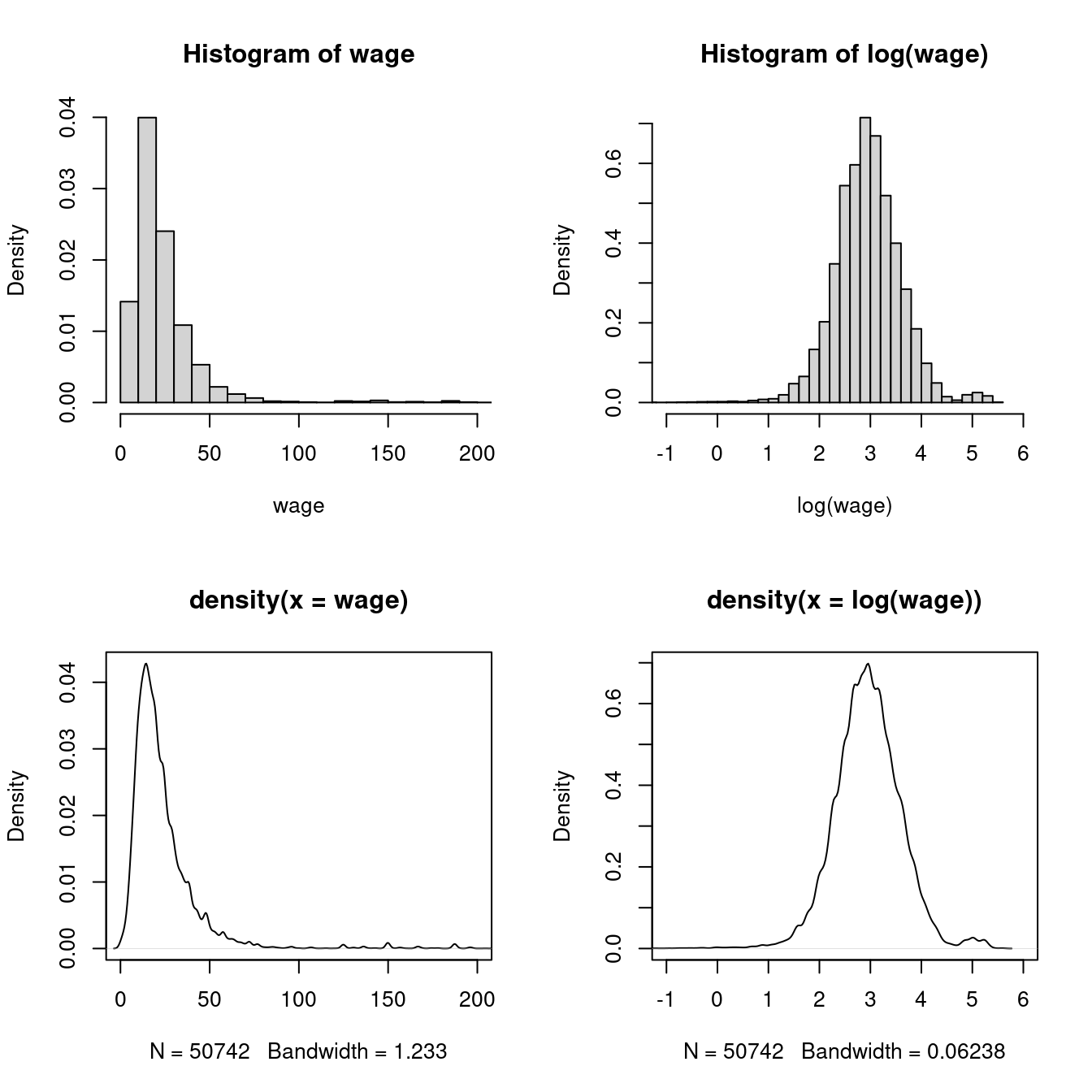
[1] 4.320157 30.370331[1] -0.6990539 11.8566367In econometrics, statistics, and many programming languages including R, \log(\cdot) is commonly used to denote the natural logarithm (base e).
Note: On a pocket calculator, use LN to calculate the natural logarithm \log(\cdot)=\log_e(\cdot). If you use LOG, you will calculate the logarithm with base 10, i.e., \log_{10}(\cdot), which will give you a different result. The relationship between these logarithms is \log_{10}(x) = \log_{e}(x)/\log_{e}(10).
2.7 Bivariate Statistics
For a bivariate sample (Y_1, Z_1), \ldots, (Y_n, Z_n), we can compute cross moments that describe the relationship between the two variables. The (r,s)-th sample cross moment is defined as: \overline{Y^rZ^s} = \frac{1}{n} \sum_{i=1}^n Y_i^r Z_i^s. The most important cross moment is the (1,1)-th sample cross moment, or simply the first sample cross moment: \overline{YZ} = \frac{1}{n} \sum_{i=1}^n Y_i Z_i. The central sample cross moments are defined as: \frac{1}{n} \sum_{i=1}^n (Y_i - \overline{Y})^r(Z_i - \overline{Z})^s.
Covariance and Correlation
The (1,1)-th central sample cross moment leads to the sample covariance: \widehat{\sigma}_{YZ} = \frac{1}{n} \sum_{i=1}^n (Y_i - \overline{Y})(Z_i - \overline{Z}) = \overline{YZ} - \overline{Y} \cdot \overline{Z}. Similar to the univariate case, we can define the adjusted sample covariance: s_{YZ} = \frac{1}{n-1} \sum_{i=1}^n (Y_i - \overline{Y})(Z_i - \overline{Z}) = \frac{n}{n-1}\widehat{\sigma}_{YZ}. The sample correlation coefficient is the standardized sample covariance: r_{YZ} = \frac{s_{YZ}}{s_Y s_Z} = \frac{\sum_{i=1}^n (Y_i - \overline{Y})(Z_i - \overline{Z})}{\sqrt{\sum_{i=1}^n (Y_i - \overline{Y})^2}\sqrt{\sum_{i=1}^n (Z_i - \overline{Z})^2}} = \frac{\widehat{\sigma}_{YZ}}{\widehat{\sigma}_Y \widehat{\sigma}_Z}.
If the sample is i.i.d., both \widehat{\sigma}_{YZ} and s_{YZ} are consistent estimators for the population covariance \sigma_{YZ} = Cov(Y,Z) = E[(Y - E[Y])(Z - E[Z])]. The adjusted sample covariance s_{YZ} is unbiased, while \widehat{\sigma}_{YZ} is biased but has a lower sampling variance. Similarly, the sample correlation coefficient is a consistent estimator for the population correlation coefficient \rho_{YZ} = Corr(Y,Z) = \frac{Cov(Y,Z)}{\sqrt{Var(Y)Var(Z)}}.
To compute these quantities for a bivariate sample collected in the vectors Y and Z, use cov(Y,Z) for the adjusted sample covariance and cor(Y,Z) for the sample correlation.
2.8 Moment Matrices
Consider a multivariate dataset \boldsymbol X_1, \ldots, \boldsymbol X_n, such as the following subset of the cps dataset:
dat = data.frame(wage, edu, fem)Mean Vector
The sample mean vector \overline{\boldsymbol X} contains the sample means of the k variables and is defined as \overline{\boldsymbol X} = \frac{1}{n} \sum_{i=1}^n \boldsymbol X_i.
For i.i.d. samples, the sample mean vector is a consistent estimator for the population mean vector E[\boldsymbol X].
colMeans(dat) wage edu fem
23.9026619 13.9246187 0.4257223 Covariance Matrix
The sample covariance matrix \widehat{\Sigma} is the k \times k matrix given by \widehat{\Sigma} = \frac{1}{n} \sum_{i=1}^n (\boldsymbol X_i - \overline{\boldsymbol X})(\boldsymbol X_i - \overline{\boldsymbol X})'.
Its elements \widehat \sigma_{h,l} represent the pairwise sample covariance between variables h and l: \widehat \sigma_{h,l} = \frac{1}{n} \sum_{i=1}^n (X_{ih} - \overline{X_h})(X_{il} - \overline{X_l}), \quad \overline{X_h} = \frac{1}{n} \sum_{i=1}^n X_{ih}.
The adjusted sample covariance matrix S is defined as S = \frac{1}{n-1} \sum_{i=1}^n (\boldsymbol X_i - \overline{\boldsymbol X})(\boldsymbol X_i - \overline{\boldsymbol X})'
Its elements s_{h,l} are the adjusted sample covariances, with main diagonal elements s_{h}^2 = s_{h,h} being the adjusted sample variances: s_{h,l} = \frac{1}{n-1} \sum_{i=1}^n (X_{ih} - \overline{X_h})(X_{il} - \overline{X_l}).
If the sample is i.i.d., both \widehat{\Sigma} and S are consistent estimators for the population covariance matrix \Sigma = Var(\boldsymbol X)= E[(\boldsymbol X - E[\boldsymbol X])(\boldsymbol X - E[\boldsymbol X])']. The adjusted covariance matrix S is unbiased, while \widehat{\Sigma} is biased but has lower sampling variance.
## Adjusted sample covariance matrix
cov(dat)
wage edu fem
wage 428.948332 21.82614057 -1.66314777
edu 21.826141 7.53198925 0.06037303
fem -1.663148 0.06037303 0.24448764Correlation Matrix
The sample correlation coefficient between the variables h and l is the standardized sample covariance: r_{h,l} = \frac{s_{h,l}}{s_h s_l} = \frac{\sum_{i=1}^n (X_{ih} - \overline{X_h})(X_{il} - \overline{X_l})}{\sqrt{\sum_{i=1}^n (X_{ih} - \overline{X_h})^2}\sqrt{\sum_{i=1}^n (X_{il} - \overline{X_l})^2}} = \frac{\widehat \sigma_{h,l}}{\widehat \sigma_h \widehat \sigma_l}.
These coefficients form the sample correlation matrix R, expressed as: R = D^{-1} S D^{-1}, where D is the diagonal matrix of adjusted sample standard deviations: D = diag(s_1, \ldots, s_k) = \begin{pmatrix} s_1 & 0 & \ldots & 0 \\ 0 & s_2 & \ldots & 0 \\ \vdots & & \ddots & \vdots \\ 0 & 0 & \ldots & s_k \end{pmatrix}
The matrices \widehat{\Sigma}, S, and R are symmetric.
cor(dat) wage edu fem
wage 1.0000000 0.38398973 -0.16240519
edu 0.3839897 1.00000000 0.04448972
fem -0.1624052 0.04448972 1.00000000We find a strong positive correlation between wage and edu, a substantial negative correlation between wage and fem, and a negligible correlation between edu and fem.