In applied regression analysis, we often want to assess whether a regressor has a statistically significant relationship with the outcome variable (conditional on other regressors).
6.1 t-Test
The most common hypothesis test evaluates whether a regression coefficient equals zero:
H_0: \beta_j = 0 \quad \text{vs.} \quad H_1: \beta_j \ne 0.
This corresponds to testing whether the marginal effect of the regressor X_{ij} on the outcome Y_i is zero, holding other regressors constant.
We use the t-statistic:
T_j = \frac{\widehat{\beta}_j}{se(\widehat{\beta}_j)},
where se(\widehat{\beta}_j) is a standard error.
You may use the classical standard error if you have strong evidence that the errors are homoskedastic. However, in most economic applications, heteroskedasticity-robust standard errors are more reliable.
Under the null, T_j follows approximately a t_{n-k} distribution. We reject H_0 at the significance level \alpha if:
|T_j| > t_{n-k,1-\alpha/2}.
This decision rule is equivalent to checking whether the confidence interval for \beta_j includes 0:
Reject H_0 if 0 lies outside the 1-\alpha confidence interval
Fail to reject (accept) H_0 if 0 lies inside the 1-\alpha confidence interval
6.2 p-Value
The p-value is a criterion to reach a hypothesis test decision conveniently: \begin{align*}
\text{reject} \ H_0 \quad &\text{if p-value} < \alpha \\
\text{do not reject} \ H_0 \quad &\text{if p-value} \geq \alpha
\end{align*}
Formally, the p-value represents the probability of observing a test statistic as extreme or more extreme than the one we computed, assuming H_0 is true. For the t-test, the p-value is:
p\text{-value} = P( |T| > |T_j| \mid H_0 \ \text{is true})
Here, T is a random variable following the null distribution Z\sim t_{n-k}, and T_j is the observed value of the test statistic.
Another way of representing the p-values of a t-test is:
p\text{-value} = 2(1 - F_{t_{n-k}}(|T_j|)),
where F_{t_{n-k}} is the cumulative distribution function (CDF) of the t_{n-k}-distribution.
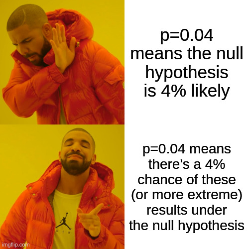
A common misinterpretation of p-values is treating them as the probability that the null hypothesis is being true. This is incorrect. The p-value is not a statement about the probability of the null hypothesis itself.
The correct interpretation is that the p-value represents the probability of observing a test statistic at least as extreme as the one calculated from our sample, assuming that the null hypothesis is true.
In other words, a p-value of 0.04 means:
❌ NOT “There’s a 4% chance that the null hypothesis is true”
✓ INSTEAD “If the null hypothesis were true, there would be a 4% chance of observing a test statistic this extreme or more extreme”
Small p-values indicate that the observed data would be unlikely under the null hypothesis, which leads us to reject the null in favor of the alternative. However, they do not tell us the probability that our alternative hypothesis is correct, nor do they directly measure the magnitude or significance of the marginal effect.
Relation to Confidence Intervals:
Zero lies outside the (1-\alpha) confidence interval for \beta_j if and only if the p-value for testing H_0: \beta_j = 0 is less than \alpha.
6.3 Significance Stars
Regression tables often use asterisks to indicate levels of statistical significance. Stars summarize statistical significance by comparing the t-statistic to critical values (or equivalently, the p-value or whether 0 is covered by the confidence interval)
0 outside \small I_{0.95}, but inside \small I_{0.99}
Significance Stars Convention
Note that most economists use the following significance levels: *** for 1%, ** for 5%, and * for 10%. In this lecture, we follow the convention of R, which uses the significance levels *** for 0.1%, ** for 1%, and * for 5%.
Regression Tables
Let’s revisit the regression of wage on education and female.
All p-values are super small: 2.2e-16 means 2.2 \cdot 10^{-16} (15 zeros after the decimal point, followed by 22).
Let’s also revisit the CASchools dataset and examine four regression models on test scores.
library(AER)data(CASchools, package ="AER")CASchools$STR=CASchools$students/CASchools$teachersCASchools$score=(CASchools$read+CASchools$math)/2fitA=feols(score~STR, data =CASchools)fitB=feols(score~STR+english, data =CASchools)fitC=feols(score~STR+english+lunch, data =CASchools)fitD=feols(score~STR+english+lunch+expenditure, data =CASchools)
Models A–C: The coefficient is negative and statistically significant. However, when using robust standard errors, the coefficient in model B becomes only weakly significant.
Model D: The coefficient remains negative but becomes insignificant when controlling for expenditure.
As discussed earlier, expenditure is a bad control in this context and should not be used to estimate a ceteris paribus effect of class size on test scores.
6.4 Testing for Heteroskedasticity: Breusch-Pagan Test
Classical standard errors should only be used if you have statistical evidence that the errors are homoskedastic. A statistical test for this is the Breusch-Pagan Test.
Under homoskedasticity, the variance of the error term is constant and does not depend on the values of the regressors:
Var(u_i \mid \boldsymbol X_i) = \sigma^2 \quad \text{(constant)}.
To test this assumption, we perform an auxiliary regression of the squared residuals on the original regressors:
\widehat u_i^2 = \boldsymbol X_i' \boldsymbol \gamma + v_i, \quad i = 1, \ldots, n,
where:
\widehat u_i are the OLS residuals from the original model,
\boldsymbol \gamma are auxiliary coefficients,
v_i is the error term in the auxiliary regression.
If homoskedasticity holds, the regressors should not explain any variation in \widehat u_i^2, which means the auxiliary regression should have low explanatory power.
Let R^2_{\text{aux}} be the R-squared from this auxiliary regression. Then, the Breusch–Pagan (BP) test statistic is:
BP = n \cdot R^2_{\text{aux}}
Under the null hypothesis of homoskedasticity,
H_0: Var(u_i \mid \boldsymbol X_i) = \sigma^2,
the test statistic follows an asymptotic chi-squared distribution with k-1 degrees of freedom:
BP \overset{d}{\rightarrow} \chi^2_{k-1}
We reject H_0 at significance level \alpha if:
BP > \chi^2_{1-\alpha,\,k-1}.
This basic variant of the BP test is Koenker’s version of the test. Other variants include further nonlinear transformations of the regressors.
In R, the test is implemented via the bptest() function from the AER package. Unfortunately, the bptest() function does not work directly with feols objects, so we need to estimate the model first with lm():
fit=lm(wage~education+female, data =cps)bptest(fit)
    studentized Breusch-Pagan test

data:  fit
BP = 1070.3, df = 2, p-value < 2.2e-16
In the wage regression the BP test clearly rejects H_0, which is strong statistical evidence that the errors are heteroskedastic.
    studentized Breusch-Pagan test

data:  lm(score ~ STR + english, data = CASchools)
BP = 29.501, df = 2, p-value = 3.926e-07
lm(score~STR+english+lunch, data =CASchools)|>bptest()
    studentized Breusch-Pagan test

data:  lm(score ~ STR + english + lunch, data = CASchools)
BP = 9.9375, df = 3, p-value = 0.0191
lm(score~STR+english+lunch+expenditure, data =CASchools)|>bptest()
    studentized Breusch-Pagan test

data:  lm(score ~ STR + english + lunch + expenditure, data = CASchools)
BP = 5.9649, df = 4, p-value = 0.2018
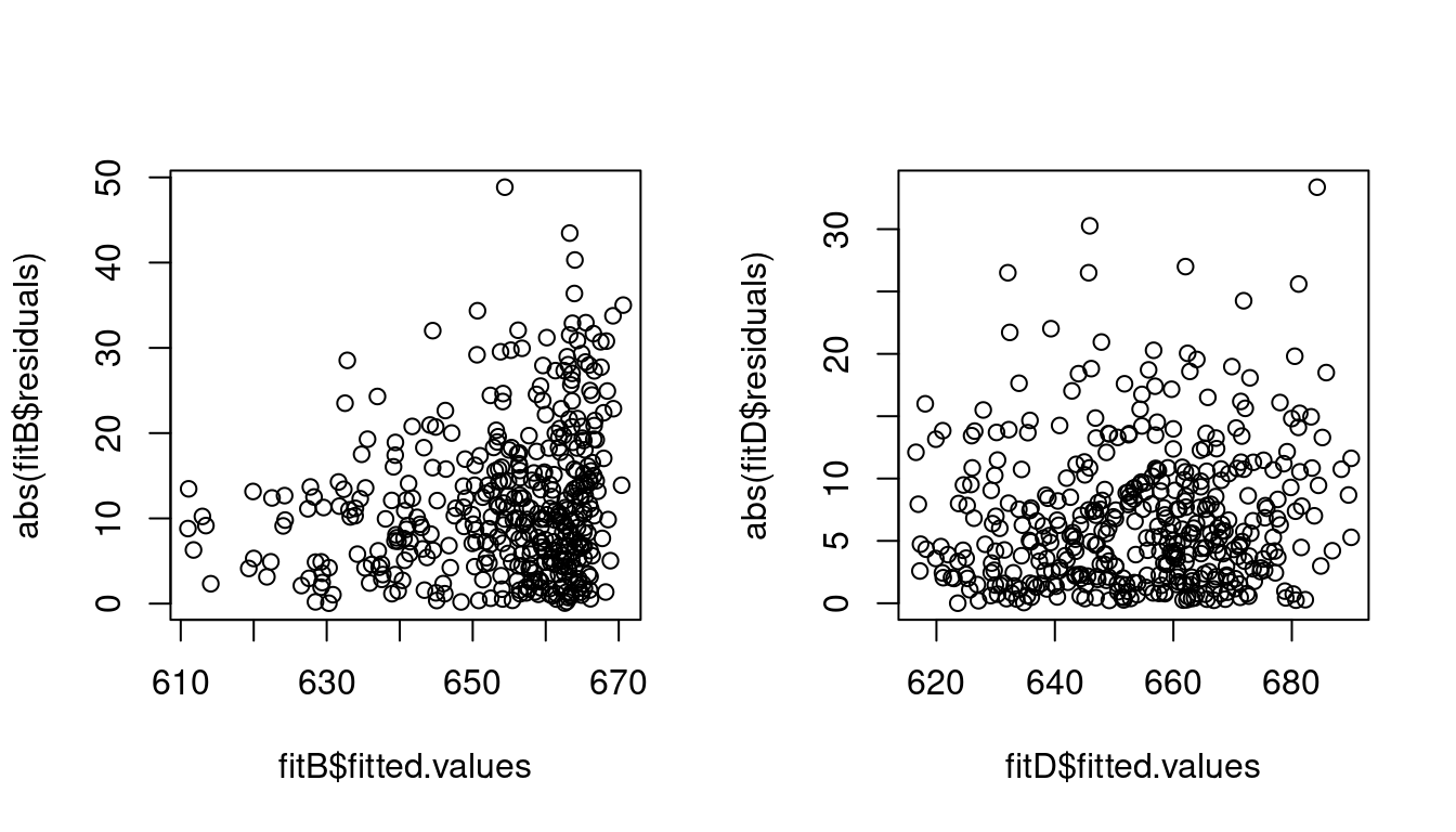
In the regression of score on STR and english there is strong statistical evidence that errors are heteroskedastic, whereas when adding lunch and expenditure there is no evidence of heteroskedasticity. See the difference in the absolute residuals against fitted values plot:
The heteroskedasticity pattern in model (2) likely occurred because of a nonlinear dependence of the omitted variables lunch and expenditure with the included regressors STR and english. The inclusion of these variables in model (4) eliminated the heteroskedasticity (apparent heteroskedasticity). Therefore, heteroskedasticity is sometimes a sign of model misspecification.
6.5 Testing for Normality: Jarque–Bera Test
A general property of a normally distributed variable is that it has zero skewness and kurtosis of three. In the Gaussian regression model, this implies:
u_i|\boldsymbol X_i \sim \mathcal{N}(0, \sigma^2) \quad \Rightarrow \quad E[u_i^3] = 0, \quad E[u_i^4] = 3 \sigma^4.
The sample skewness and sample kurtosis of the OLS residuals are:
\widehat{\text{ske}}(\widehat{\boldsymbol u}) = \frac{1}{n \widehat \sigma_{\widehat u}^3} \sum_{i=1}^n \widehat u_i^3, \quad
\widehat{\text{kur}}(\widehat{\boldsymbol u}) = \frac{1}{n \widehat \sigma_{\widehat u}^4} \sum_{i=1}^n \widehat u_i^4
A joint test for normality — assessing both skewness and kurtosis — is the Jarque–Bera (JB) test, with statistic:
JB = n \left( \frac{1}{6} \widehat{\text{ske}}(\widehat{\boldsymbol u})^2 + \frac{1}{24} (\widehat{\text{kur}}(\widehat{\boldsymbol u}) - 3)^2 \right)
Under the null hypothesis of normal errors, this test statistic is asymptotically chi-squared distributed:
JB \overset{d}{\to} \chi^2_2
We reject H_0 at level \alpha if:
JB > \chi^2_{1-\alpha,\,2}.
In R, we can apply the test using the moments package:
    Jarque-Bera Normality Test

data:  fitD$residuals
JB = 8.9614, p-value = 0.01133
alternative hypothesis: greater
Although the Breusch–Pagan test does not reject homoskedasticity for fitD (so classical standard errors are valid asymptotically), the JB rejects the null hypothesis of normal errors at the 5% level and provides statistical evidence that the errors are not normally distributed.
This means that exact inference based on t-distributions is not valid in finite samples, and confidence intervals or t-test results give only large sample approximations.
In econometrics, asymptotic large sample approximations have become the convention because exact finite sample inference is rarely feasible.
6.6 Joint Hypothesis Testing
So far, we’ve tested whether a single coefficient is zero. But often we want to test multiple restrictions simultaneously, such as whether a group of variables has a joint effect.
The joint exclusion hypothesis formulates the null hypothesis that a set of coefficients or linear combinations of coefficients are equal to zero:
H_0: \boldsymbol{R}\boldsymbol{\beta} = \boldsymbol{0}
where:
\boldsymbol{R} is a q \times k restriction matrix,
\boldsymbol{0} is the q \times 1 vector of zeros,
q is the number of restrictions.
Consider for example the score on STR regression with interaction effects:
\text{score}_i = \beta_1 + \beta_2 \text{STR}_i + \beta_3 \text{HiEL}_i + \beta_4 \text{STR}_i \cdot \text{HiEL}_i + u_i.
## Create dummy variable for high proportion of English learnersCASchools$HiEL=(CASchools$english>=10)|>as.numeric()fitE=feols(score~STR+HiEL+STR:HiEL, data =CASchools, vcov ="hc1")fitE|>summary()
The model output reveals that none of the individual t-tests reject the null hypothesis that the individual coefficients are zero.
However, these results are misleading because the true marginal effects are a mixture of these coefficients:
\frac{\partial E[\text{score}_i \mid \boldsymbol X_i]}{\partial \text{STR}_i} = \beta_2 + \beta_4 \cdot \text{HiEL}_i.
Therefore, to test if STR has an effect on score, we need to test the joint hypothesis:
H_0: \beta_2 = 0 \quad \text{and} \quad \beta_4 = 0.
In terms of the multiple restriction notation H_0: \boldsymbol{R} \boldsymbol{\beta} = \boldsymbol{0}, we have
\boldsymbol{R} = \begin{pmatrix}
0 & 1 & 0 & 0 \\
0 & 0 & 0 & 1
\end{pmatrix}.
Similarly, the marginal effects of HiEL is:
\frac{\partial E[\text{score}_i \mid \boldsymbol X_i]}{\partial \text{HiEL}_i} = \beta_3 + \beta_4 \cdot \text{STR}_i.
We test the joint hypothesis that \beta_3 = 0 and \beta_4 = 0:
\boldsymbol{R} = \begin{pmatrix}
0 & 0 & 1 & 0 \\
0 & 0 & 0 & 1
\end{pmatrix}.
Wald Test
The Wald test is based on the Wald distance:
\boldsymbol{d} = \boldsymbol{R} \widehat{\boldsymbol{\beta}},
which measures how far the estimated coefficients deviate from the hypothesized restrictions.
The covariance matrix of the Wald distance is: Var(\boldsymbol{d} | \boldsymbol X) = \boldsymbol{R} Var(\widehat{\boldsymbol \beta} | \boldsymbol X) \boldsymbol R', which can be estimated as:
\widehat{Var}(\boldsymbol{d} \mid \boldsymbol X) = \boldsymbol{R} \widehat{\boldsymbol{V}} \boldsymbol{R}'.
The Wald statistic is the squared, variance-standardized distance:
W = \boldsymbol{d}' (\boldsymbol{R} \widehat{\boldsymbol{V}} \boldsymbol{R}')^{-1} \boldsymbol{d},
where \widehat{\boldsymbol{V}} is a consistent estimator of the covariance matrix of \widehat{\boldsymbol{\beta}} (e.g., HC1 robust: \widehat{\boldsymbol{V}} = \widehat{\boldsymbol{V}}_{hc1}).
Under the null hypothesis, and assuming (A1)–(A4), the Wald statistic has an asymptotic chi-squared distribution:
W \overset{d}{\to} \chi^2_q,
where q is the number of restrictions.
The null is rejected if W > \chi^2_{1-\alpha, q}.
F-test
The Wald test is an asymptotic size-\alpha-test under (A1)–(A4). Even if normality and homoskedasticity hold true as well, the Wald test is still only asymptotically valid, i.e.:
\lim_{n \to \infty} P( \text{Wald test rejects} \ H_0 | H_0 \ \text{true} ) = \alpha.
The F-test is the small sample correction of the Wald test. It is based on the same distance as the Wald test, but it is scaled by the number of restrictions q:
F = \frac{W}{q} = \frac{1}{q} (\boldsymbol R\widehat{\boldsymbol \beta} - \boldsymbol r)'(\boldsymbol R \widehat{\boldsymbol V} \boldsymbol R')^{-1} (\boldsymbol R\widehat{\boldsymbol \beta} - \boldsymbol r).
Under the restrictive assumption that the Gaussian regression model holds, and if \widehat{\boldsymbol V} = \widehat{\boldsymbol V}_{hom} is used, it can be shown that
F \sim F_{q;n-k}
for any finite sample size n. Here, F_{q;n-k} is the F-distribution with q degrees of freedom in the numerator and n-k degrees of freedom in the denominator.
The test decision for the F-test: \begin{align*}
\text{do not reject} \ H_0 \quad \text{if} \ &F \leq F_{(1-\alpha,q,n-k)}, \\
\text{reject} \ H_0 \quad \text{if} \ &F > F_{(1-\alpha,q,n-k)},
\end{align*} where F_{(p,m_1,m_2)} is the p-quantile of the F distribution with m_1 degrees of freedom in the numerator and m_2 degrees of freedom in the denominator.
F- and Chi-squared distribution
Similar to how the t-distribution t_{n-k} approaches the standard normal as sample size increases, we have q \cdot F_{q;n-k} \to \chi^2_{q} as n \to \infty. Therefore, the F-test and Wald test become asymptotically equivalent and lead to identical statistical conclusions in large samples. For single constraint (q=1) hypotheses of the form H_0: \beta_j = 0, the F-test is equivalent to a two-sided t-test.
The F-test can be viewed as a finite-sample correction of the Wald test. It tends to be more conservative than the Wald test in small samples, meaning that rejection by the F-test generally implies rejection by the Wald test, but not necessarily vice versa. Due to this more conservative nature, which helps control false rejections (Type I errors) in small samples, the F-test is often preferred in practice.
F-tests in R
The function wald() from the fixest package performs an F-test:
Wald test, H0: joint nullity of HiEL and STR:HiEL
 stat = 89.9, p-value < 2.2e-16, on 2 and 416 DoF, VCOV: Heteroskedasticity-robust.
The hypotheses that STR and HiEL have no effect on score can be clearly rejected.
Another research question is whether the effect of STR on score is zero only for the subgroup of schools with a high proportion of English learners (HiEL = 1). In this case, the marginal effect is:
\frac{\partial E[\text{score}_i \mid \boldsymbol X_i, \text{HiEL}_i = 1]}{\partial \text{STR}_i} = \beta_2 + \beta_4 \cdot 1,
and the null hypothesis is:
H_0: \beta_2 + \beta_4 = 0.
The corresponding restriction matrix is:
\boldsymbol{R} = \begin{pmatrix}
0 & 1 & 0 & 1
\end{pmatrix},
where the number of restrictions is q=1.
The function linearHypothesis() from the AER package is more flexible for these cases:
## Define hypothesis matrix:R=matrix(c(0,1,0,1), ncol =4)linearHypothesis(fitE, hypothesis.matrix =R, test ="F", vcov. =vcovHC(fitE, type ="HC1"))
Similarly, this hypothesis can be rejected at the 0.01 level.
6.7 Jackknife Methods
Projection Matrix
Recall the vector of fitted values \widehat{\boldsymbol Y} = \boldsymbol X \widehat{\boldsymbol \beta}. Inserting the model equation gives:
\widehat{\boldsymbol Y} = \boldsymbol X \widehat{\boldsymbol \beta} = \underbrace{\boldsymbol X (\boldsymbol X'\boldsymbol X)^{-1} \boldsymbol X'}_{=\boldsymbol P}\boldsymbol Y = \boldsymbol P \boldsymbol Y.
The projection matrix\boldsymbol P is also known as the influence matrix or hat matrix and maps observed values to fitted values.
Leverage Values
The diagonal entries of \boldsymbol P, given by
h_{ii} = \boldsymbol X_i'(\boldsymbol X' \boldsymbol X)^{-1} \boldsymbol X_i,
are called leverage values or hat values and measure how far away the regressor values of the i-th observation X_i are from those of the other observations.
Properties of leverage values:
0 \leq h_{ii} \leq 1, \quad \sum_{i=1}^n h_{ii} = k.
Leverage values h_{ii} indicate how much influence an observation \boldsymbol X_i has on the regression fit, e.g., the last observation in the following artificial dataset:
X=c(10,20,30,40,50,60,70,500)Y=c(1000,2200,2300,4200,4900,5500,7500,10000)plot(X,Y, main="OLS regression line with and without last observation")abline(lm(Y~X), col="blue")abline(lm(Y[1:7]~X[1:7]), col="red")
A low leverage implies the presence of many regressor observations similar to \boldsymbol X_i in the sample, while a high leverage indicates a lack of similar observations near \boldsymbol X_i.
An observation with a high leverage h_{ii} but a response value Y_i that is close to the true regression line \boldsymbol X_i' \boldsymbol \beta (indicating a small error u_i) is considered a good leverage point. Despite being unusual in the regressor space, this point improves estimation precision because it provides valuable information about the regression relationship in regions where data is sparse.
Conversely, a bad leverage point occurs when both h_{ii} and the error u_i are large, indicating both unusual regressor and response values. This can misleadingly impact the regression fit.
The actual error term is unknown, but standardized residuals can be used to differentiate between good and bad leverage points.
Standardized Residuals
Many regression diagnostic tools rely on the residuals of the OLS estimation \widehat u_i because they provide insight into the properties of the unknown error terms u_i.
Under the homoskedastic linear regression model (A1)–(A5), the errors are independent and have the property
Var(u_i \mid \boldsymbol X) = \sigma^2.
Since \boldsymbol P \boldsymbol X = \boldsymbol X and, therefore,
\widehat{\boldsymbol u} = (\boldsymbol I_n - \boldsymbol P)\boldsymbol Y = (\boldsymbol I_n - \boldsymbol P)(\boldsymbol X\boldsymbol \beta + \boldsymbol u) = (\boldsymbol I_n - \boldsymbol P)\boldsymbol u,
the residuals have a different property:
Var(\widehat{\boldsymbol u} \mid \boldsymbol X) = \sigma^2 (\boldsymbol I_n - \boldsymbol P).
The i-th residual satisfies
Var(\widehat u_i \mid \boldsymbol X) = \sigma^2 (1 - h_{ii}),
where h_{ii} is the i-th leverage value.
Under the assumption of homoskedasticity, the variance of \widehat u_i depends on \boldsymbol X, while the variance of u_i does not. Dividing by \sqrt{1-h_{ii}} removes the dependency:
Var\bigg( \frac{\widehat u_i}{\sqrt{1-h_{ii}}} \ \bigg| \ \boldsymbol X\bigg) = \sigma^2
The standardized residuals are defined as follows:
r_i := \frac{\widehat u_i}{\sqrt{s_{\widehat u}^2 (1-h_{ii})}}.
Standardized residuals are available using the R command rstandard().
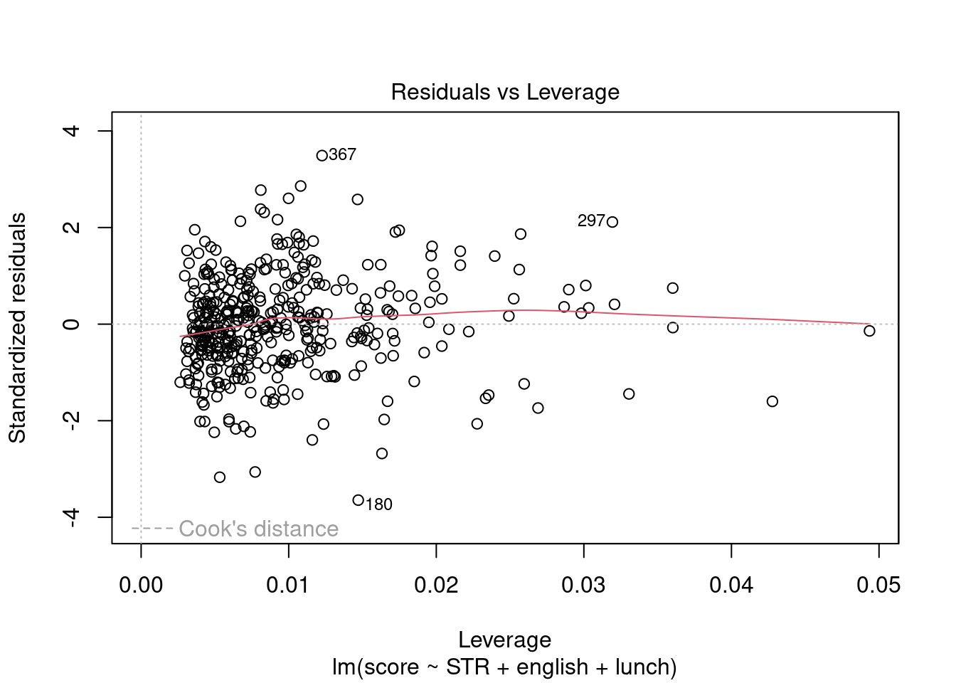
Residuals vs. Leverage Plot
Plotting standardized residuals against leverage values provides a graphical tool for detecting outliers. High leverage points have a strong influence on the regression fit. High leverage values with standardized residuals close to 0 are good leverage points, and high leverage values with large standardized residuals are bad leverage points.
fit=lm(score~STR+english+lunch, data =CASchools)plot(fit, which =5)
The plot indicates that some observations have a higher leverage value than others, but none of these have a large standardized residual, so they are not bad leverage points.
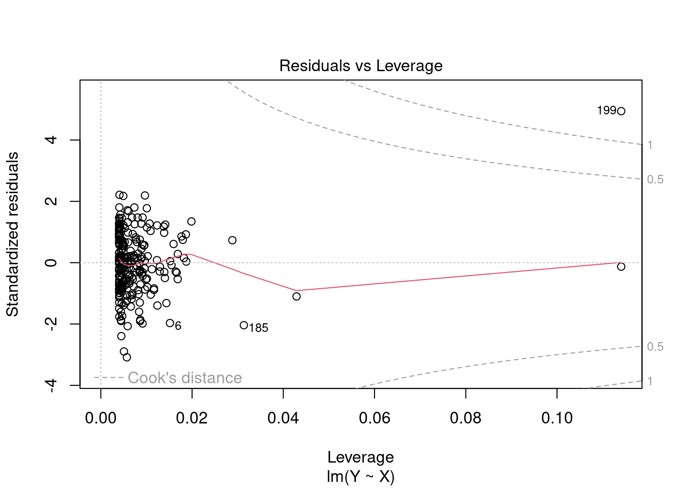
Here is an example with two high leverage points. Observation i=200 is a good leverage point and i=199 is a bad leverage point:
## simulate regressors and errorsX=rnorm(250)u=rnorm(250)## set some unusual observations manuallyX[199]=6X[200]=6u[199]=5u[200]=0## define dependent variableY=X+u## residuals vs leverage plotplot(lm(Y~X), which =5)
The plot also shows Cook’s distance thresholds. Cook’s distance for observation i is defined as
D_i = \frac{(\widehat{\boldsymbol \beta}_{(-i)} - \widehat{\boldsymbol \beta})' \boldsymbol X' \boldsymbol X (\widehat{\boldsymbol \beta}_{(-i)} - \widehat{\boldsymbol \beta})}{k s_{\widehat u}^2},
where
\widehat{\boldsymbol \beta}_{(-i)} - \widehat{\boldsymbol \beta} = (\boldsymbol X' \boldsymbol X)^{-1} \boldsymbol X_i \frac{\widehat u_i}{1-h_{ii}}.
Here, \widehat{\boldsymbol \beta}_{(-i)} is the i-th leave-one-out estimator (the OLS estimator when the i-th observation is left out).
This principle is called Jackknife because it is similar to the way a jackknife is used to cut something. The idea is to “cut” the data by removing one observation at a time and then re-estimating the model. The impact of cutting the i-th observation is proportional to \widehat u_i/(1-h_{ii}).
We should pay special attention to points outside Cook’s distance thresholds of 0.5 and 1 and check for measurement errors or other anomalies.
Jackknife Standard Errors
Recall the heteroskedasticity-robust White estimator for the meat matrix \boldsymbol \Omega = E[u_i^2 \boldsymbol X_i \boldsymbol X_i'] in the sandwich formula tor the OLS variance:
\widehat{\boldsymbol \Omega} = \frac{1}{n} \sum_{i=1}^n \widehat u_i^2 \boldsymbol X_i \boldsymbol X_i'.
If there are leverage points in the data, their presence might have a large influence on the estimation of \boldsymbol \Omega.
An alternative way of estimating the covariance matrix is to weight the observations by the leverage values:
\widehat{\boldsymbol \Omega}_{\text{jack}} = \frac{1}{n} \sum_{i=1}^n \frac{\widehat u_i^2}{(1-h_{ii})^2} \boldsymbol X_i \boldsymbol X_i'.
Observations with high leverage values have a small denominator (1-h_{ii})^2 and are therefore downweighted, which makes this estimator more robust to the influence of leverage points.
The full jackknife covariance matrix estimator is conventionally labeled as the HC3 estimator:
\widehat{\boldsymbol V}_{\text{jack}} = \widehat{\boldsymbol V}_{\text{hc3}} = \left( \boldsymbol X' \boldsymbol X \right)^{-1} \widehat{\boldsymbol \Omega}_{\text{jack}} \left( \boldsymbol X' \boldsymbol X \right)^{-1}.
There is also the HC2 estimator, which uses \widehat u_i^2(1-h_{ii}) instead of \widehat u_i^2/(1-h_{ii})^2, but this is less common.
If you have a small sample size and you are worried about influential observations, you should use the HC3 standard errors instead of the HC1 standard errors.
To display the HC3 standard errors in the regression table, you can use modelsummary(fit, vcov = "HC3").
6.8 Cluster-robust Inference
Recall that in many economic applications, observations are naturally clustered. For instance, students within the same school, workers in the same firm, or households in the same village may share common unobserved factors that induce correlation in their outcomes.
As discussed in Section 5, for clustered observations we can use the notation (\boldsymbol X_{ig}, Y_{ig}), where the linear regression equation is:
Y_{ig} = \boldsymbol X_{ig}' \boldsymbol \beta + u_{ig}, \quad i=1, \ldots, n_g, \quad g=1, \ldots, G.
Under independence across clusters but allowing for arbitrary correlation within clusters, the OLS estimator remains unbiased, but its standard variance formula is no longer valid. As we saw in Section 5, the conditional variance
Var(\widehat{\boldsymbol \beta} \mid \boldsymbol X) = (\boldsymbol X'\boldsymbol X)^{-1} \boldsymbol X' \boldsymbol D \boldsymbol X (\boldsymbol X'\boldsymbol X)^{-1}
satisfies
\boldsymbol X' \boldsymbol D \boldsymbol X = \sum_{g=1}^G E\bigg[ \Big( \sum_{i=1}^{n_g} \boldsymbol X_{ig} u_{ig} \Big) \Big( \sum_{i=1}^{n_g} \boldsymbol X_{ig} u_{ig} \Big)' \Big| \boldsymbol X \bigg].
Cluster-robust Standard Errors
When observations within clusters are correlated, using ordinary standard errors (even heteroskedasticity-robust ones) will typically underestimate the true sampling variability of the OLS estimator.
To account for within-cluster correlation, we use cluster-robust standard errors. The key insight is to estimate the middle part of the sandwich formula above by allowing for arbitrary within-cluster correlation, while maintaining the independence assumption across clusters.
This estimator, also known as the clustered sandwich estimator, allows for arbitrary correlation of errors within clusters, including both heteroskedasticity and serial correlation. Like the HC estimators, it is consistent under large-sample asymptotics.
Finite Sample Correction
Similar to the HC1 correction for heteroskedasticity, a small-sample correction for the cluster-robust estimator is commonly applied:
\widehat{\boldsymbol V}_{CR1} = \frac{G}{G-1} \cdot \frac{n-1}{n-k} \cdot \widehat{\boldsymbol V}_{CR0},
where G is the number of clusters, n is the total sample size, and k is the number of regressors.
The corresponding cluster-robust standard errors are:
se_{CR1}(\widehat{\beta}_j) =
\sqrt{[\widehat{\boldsymbol V}_{CR1}]_{jj}}.
When to Cluster
You should use cluster-robust standard errors when:
There’s a clear grouping structure in your data (schools, villages, firms, etc.)
You expect errors to be correlated within these groups
You have a sufficient number of clusters (generally at least 30-50)
Common examples include: - Student-level data clustered by school or classroom - Firm-level data clustered by industry - Individual-level data clustered by geographic region - Panel data clustered by individual or time period
Implementation in R
The CASchools dataset contains information on 420 California Schools from 45 different counties, which can be viewed as clusters.
The fixest package makes it easy to implement cluster-robust standard errors:
feols(score~STR+english, data =CASchools, cluster ="county")|>summary()
After accounting for clustering, the coefficient on STR is no longer statistically significant.
You can also use the modelsummary() function to compare the same regression with different standard errors:
fit1=feols(score~STR+english, data =CASchools)## List of standard errors:myvcov=list("IID", "HC1", "HC3", ~county)modelsummary(fit1, stars =TRUE, statistic ="conf.int", vcov =myvcov)
(1)
(2)
(3)
(4)
+ p
(Intercept)
686.032***
686.032***
686.032***
686.032***
[671.464, 700.600]
[668.875, 703.189]
[668.710, 703.354]
[654.969, 717.095]
STR
-1.101**
-1.101*
-1.101*
-1.101
[-1.849, -0.354]
[-1.952, -0.250]
[-1.960, -0.242]
[-2.584, 0.382]
english
-0.650***
-0.650***
-0.650***
-0.650***
[-0.727, -0.572]
[-0.711, -0.589]
[-0.711, -0.588]
[-0.709, -0.590]
Num.Obs.
420
420
420
420
R2
0.426
0.426
0.426
0.426
R2 Adj.
0.424
0.424
0.424
0.424
AIC
3439.1
3439.1
3439.1
3439.1
BIC
3451.2
3451.2
3451.2
3451.2
RMSE
14.41
14.41
14.41
14.41
Std.Errors
IID
HC1
HC3
by: county
Challenges with Cluster-robust Inference
The cluster-robust variance estimator relies on having a large number of clusters. With few clusters (generally G < 30), the estimator may be biased downward, leading to confidence intervals that are too narrow and overly frequent rejection of null hypotheses.
To account for high leverage points, the CR3 correction is similar to HC3 and applies a leverage adjustment at the cluster level:
\widehat{\boldsymbol V}_{CR3} = (\boldsymbol X'\boldsymbol X)^{-1} \sum_{g=1}^G \Big( \sum_{i=1}^{n_g} \boldsymbol X_{ig} \frac{\widehat u_{ig}}{1-h_{ig}} \Big) \Big( \sum_{i=1}^{n_g} \boldsymbol X_{ig} \frac{\widehat u_{ig}}{1-h_{ig}} \Big)' (\boldsymbol X'\boldsymbol X)^{-1}.